Recall that the impulse response of \(\dot {x}=Ax+Bu\), \(y=Cx+Du\) is defined as the derivative of the step response and if \(D=0\), it equals \(C\e ^{At}B\).
Remark7.1. In the case where \(m=p=1\), the impulse response is the output when the input equals the Dirac delta (which
engineers refer to as a unit impulse) hence the term impulse response. We will not be using this characterization though (since we don’t want to get into the Dirac delta).
Remark7.2. The following often provides a convenient method to calculate the impulse
response directly. If \(m=1\) (i.e. \(B\) is a vector) and \(D=0\), then the solution of the initial value problem
\[ \dot {x}=Ax,\qquad x(0)=B,\qquad y=Cx, \]
is \(y(t)=C\e ^{At}B\) and therefore equals the impulse response. If \(m>1\), then we can calculate the impulse response column-by-column in this way by choosing \(x(0)\) subsequently to be each of the columns of \(B\) (although the
computational advantage of not having to calculate \(\e ^{At}\) disappears when \(m\) becomes larger).
Remark7.3. Another method to calculate the impulse response is to inverse Laplace transform the transfer
function (which especially for higher order equations is easy to obtain).
7.1 Examples
Example7.4. The impulse response of the first order scalar differential equation
\[ \dot {x}+x=u,\quad y=x, \]
is easy to calculate using the formula \(h(t)=C\e ^{At}B\). We clearly have \(A=-1\), \(B=C=1\), \(D=0\) so that
\[ h(t)=\e ^{-t}. \]
Example7.5. We calculate the impulse response of the second order scalar differential
equation
\[ \ddot {q}+3\dot {q}+2q=2u,\qquad y=q, \]
by determining its step response and differentiating this. We therefore consider
A particular solution is \(q=1\). The homogeneous equation is \(\ddot {q}+3\dot {q}+2q=0\), which has characteristic polynomial \(s^2+3s+2\), which has roots \(-1\) and \(-2\) and therefore we obtain the general solution of our original equation
\[ q(t)=1+a\e ^{-t}+b\e ^{-2t}. \]
This gives
\[ \dot {q}(t)=-a\e ^{-t}-2b\e ^{-2t}, \]
so that the initial conditions give
\[ 1+a+b=0,\qquad -a-2b=0. \]
Solving this system of equations gives \(a=-2\), \(b=1\). With the above \(q\) we have \(h(t)=H'(t)=\dot {q}\), so that
\[ h(t)=2\e ^{-t}-2\e ^{-2t}. \]
Example7.6. We calculate the impulse response from Example 7.5 using
the transfer function. We can immediately read off the transfer function as
\[ G(s)=\frac {2}{s^2+3s+2}. \]
Using partial fractions we see that this equals
\[ \frac {2}{s+1}-\frac {2}{s+2}. \]
We recognize this as the Laplace transform of
\[ 2\e ^{-t}-2\e ^{-2t}, \]
which therefore must be the impulse response.
Example7.7. We calculate the impulse response from Example 7.5 using
Remark 7.2. With the usual state \(x=\sbm {y\\\dot {y}}\) for a second order differential equation, we have
\[ B=\bbm {0\\2}. \]
The differential equation \(\dot {x}=Ax\) from Remark 7.2 is simply the first order form of the homogeneous equation
\[ \ddot {q}+3\dot {q}+2q=0. \]
The initial condition \(x(0)=B\) is the first order form of \(q(0)=0\), \(\dot {q}(0)=2\). Therefore we have to solve
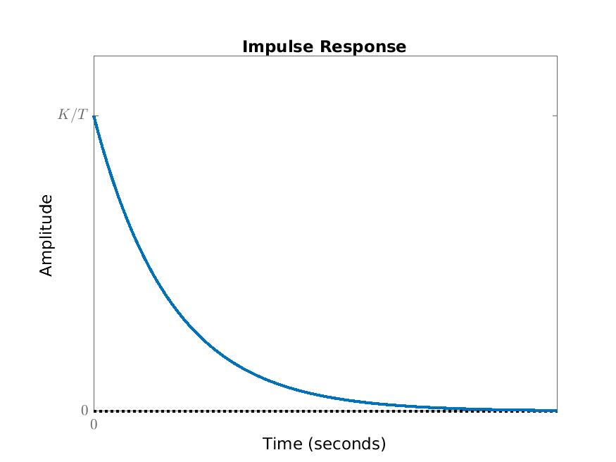
which equals \(h(t)=K\e ^{-t/T}\) (either by scaling and using Example 7.4 or a direct calculation similar to Example 7.4). The shape doesn’t
depend on \(T\) and \(K\) since these scale out.
Figure 7.1: Impulse response for first order system.
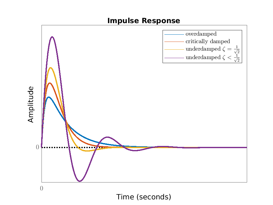
for various values of \(\zeta \) (the shape doesn’t depend on \(T\) and \(K\) since these scale out).
(a) Impulse response for second order scalar differential equation (\(y=q\)).
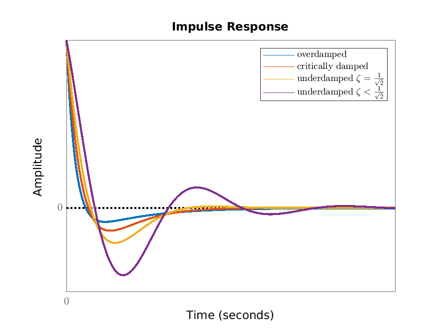
(b) Impulse response for second order scalar differential equation (\(y=\dot {q}\)).
Figure 7.2: Impulse responses for second order scalar differential equations.
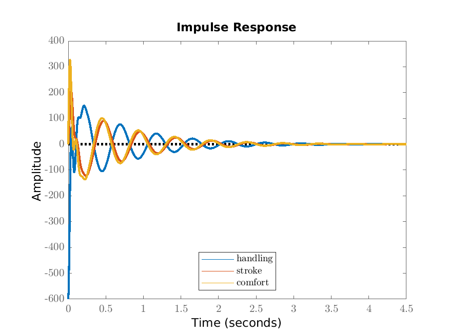
7.3 Case study: a suspension system*
We consider the fixed structure suspension system. In Figure 7.3 we give the impulse response from the road velocity to each of the three performance outputs. Here we have chosen
values for the various physical parameters as in an earlier chapter. The road velocity being the Dirac delta correponds to the road profile being the Heaviside step function. This corresponds for example to mounting a curb.
From Figure 7.3 we see that the outputs are oscillatory (as expected) and the amplitude of the oscillations is significant for about two seconds.
Figure 7.3: Impulse responses for the three outputs \(z_1\), \(z_2\) and \(z_3\) for reasonable (non-optimal) values of \(d\) and \(k_s\).