Chapter 15 Observability II
15.1 Examples
-
Example 15.1. Consider the second order scalar differential equation
\[ \ddot {q}(t)+2\zeta \dot {q}(t)+q(t)=0,\qquad y(t)=q(t), \]
where \(\zeta \geq 0\), the state is \(x=\sbm {q\\\dot {q}}\). Hence
\[ A=\bbm {0&1\\-1&-2\zeta },\qquad C=\bbm {1&0}. \]
We can see from the definition that this system is observable. If \(q(t)=0\) for all \(t\geq 0\), then by differentiating we have that \(\dot {q}(t)=0\) for all \(t\geq 0\) and therefore \(x(t)=0\) for all \(t\geq 0\). In particular \(x(0)=0\) and therefore the only unobservable state is zero.
-
Example 15.2. Consider the second order scalar differential equation
\[ \ddot {q}(t)+2\zeta \dot {q}(t)+q(t)=0,\qquad y(t)=\dot {q}(t), \]
where \(\zeta \geq 0\), the state is \(x=\sbm {q\\\dot {q}}\). Hence
\[ A=\bbm {0&1\\-1&-2\zeta },\qquad C=\bbm {0&1}. \]
We can show from the definition that this system is observable, but this is slightly more complicated than it was for Example 15.1. Assume that \(y(t)=0\) for all \(t\geq 0\), i.e. that \(\dot {q}(t)=0\) for all \(t\geq 0\). Then \(\ddot {q}(t)=0\) for all \(t\geq 0\). From the differential equation we then obtain that \(q(t)=0\) for all \(t\geq 0\). Hence \(x(t)=0\) for all \(t\geq 0\) and in particular \(x(0)=0\). We see that zero is the only state which is unobservable and therefore that the system is observable.
We can also consider the Kalman observability matrix. We have
\[ CA=\bbm {-1&-2\zeta }, \]
so that
\[ \bbm {C\\CA}=\bbm {0&1\\-1&-2\zeta }, \]
which has determinant \(1\), which is nonzero, and therefore is invertible and therefore is injective. Hence we have observability.
The Hautus observability matrix is
\[ \bbm {s&-1\\1&s+2\zeta \\0&1}. \]
Picking the second and last rows gives the matrix
\[ \bbm {1&s+2\zeta \\0&1}, \]
which is upper-triangular with nonzero elements on the diagonal and is therefore invertible (no matter what \(s\in \mC \) is). It follows that the Hautus observability matrix is injective for all \(s\in \mC \) and from this we see that the system is observable.
If \(\zeta >0\), then \(A\) is asymptotically stable and we can consider the infinite-time observability Gramian. The observation Lyapunov equation is (using that \(S\) is symmetric)
\[ \bbm {0&-1\\1&-2\zeta } \bbm {S_1&S_0\\S_0&S_2} +\bbm {S_1&S_0\\S_0&S_2} \bbm {0&1\\-1&-2\zeta } +\bbm {0\\1}\bbm {0&1}=\bbm {0&0\\0&0}, \]
which is
\[ \bbm {-2S_0&-S_2+S_1-2\zeta S_0\\ -S_2+S_1-2\zeta S_0&2S_0-4\zeta S_2+1}=\bbm {0&0\\0&0}. \]
The top-left corner gives that \(S_0=0\). The bottom-right corner then gives that \(S_2=\frac {1}{4\zeta }\). The off-diagonal entry then gives \(S_1=\frac {1}{4\zeta }\). Hence
\[ S=\frac {1}{4\zeta }\bbm {1&0\\0&1}. \]
Since \(S\) is invertible, we see that the system is observable.
-
Example 15.3. We can use the infinite-time observability Gramian from Example 15.2 to compute \(\int _0^\infty |h(t)|^2\,dt\) where \(h\) is the impulse response of the system
\[ \ddot {q}(t)+2\zeta \dot {q}(t)+q(t)=u(t),\qquad y(t)=\dot {q}(t), \]
where \(\zeta >0\). By Remark 14.9 we have
\[ \int _0^\infty |h(t)|^2\,dt=\ipd {SB}{B}, \]
where
\[ S=\frac {1}{4\zeta }\bbm {1&0\\0&1},\qquad B=\bbm {0\\1}, \]
so we have
\[ \int _0^\infty |h(t)|^2\,dt=\frac {1}{4\zeta }. \]
In particular, we see that this gets smaller the larger \(\zeta \) is.
-
Example 15.4. We use the Kalman observability matrix to show that the state-output system with
\[ A=\bbm {1&1&1\\0&1&1\\0&0&1},\qquad C=\bbm {1&0&0}, \]
is observable. We have that the Kalman observability matrix is
\[ \bbm {C\\CA\\CA^2}=\bbm {1&0&0\\1&1&1\\1&2&3}. \]
Developing by the first row, we see that the determinant of this matrix is 1. Therefore the Kalman observability matrix is invertible and therefore injective. It follows that the system is observable.
15.2 Case study: control of a tape drive*
Since we measure the whole state, it is clear that the state is observable from the measurement. To make tape drives smaller, manufacturers are looking into removing the sensor which measure the tension in the tape. This would leave only the two velocity measurements. We then have
\[ A=\bbm { -\frac {d_1}{M_1}&0&\frac {1}{M_1}\\[1mm] 0&-\frac {d_2}{M_2}&-\frac {1}{M_2}\\ -k&k&0 },\qquad C=\bbm {1&0&0\\0&1&0}. \]
The Kalman observability matrix is (since \(n=3\))
\[ \bbm {C\\CA\\CA^2}. \]
We have
\[ CA=\bbm {-\frac {d_1}{M_1}&0&\frac {1}{M_1}\\[1mm] 0&-\frac {d_2}{M_2}&-\frac {1}{M_2}}, \]
so that
\[ \bbm {C\\CA}=\bbm { 1&0&0\\0&1&0\\ -\frac {d_1}{M_1}&0&\frac {1}{M_1}\\[1mm] 0&-\frac {d_2}{M_2}&-\frac {1}{M_2} }, \]
which has rank 3 (the first three rows form a lower triangular matrix with nonzero elements on the diagonal). Therefore the Kalman observability matrix is injective (note that we didn’t even need the \(CA^2\) rows) and the system is observable. So we have observability even in the absence of measurement of the tension in the tape.
If we measure only the tension in the tape, then
\[ C=\bbm {0&0&1}, \]
and we have
\[ \bbm {C\\CA\\CA^2} =\bbm {0&0&1\\-k&k&0\\k\frac {d_1}{M_1}&-k\frac {d_2}{M_1}&\frac {-k}{M_1}-\frac {k}{M_2}}, \]
whose determinant (e.g. developing by the first row) is \(k^2\left (\frac {d_2}{M_2}-\frac {d_1}{M_1}\right )\). Therefore if \(\frac {d_2}{M_2}=\frac {d_1}{M_1}\) (in particular if \(d_1=d_2\) and \(M_1=M_2\)), then we do not have observability. More precisely we see that in this case
\[ \bbm {1\\1\\0}, \]
is in the nullspace of the Kalman observability matrix and therefore is in the unobservable subspace. This means that if the two mass-damper systems are identical, then if the velocities of the two reels are the same, we cannot determine what that common velocity is from measurement of the tension in the tape.
In concordance with Theorem 11.3 we consider observability of \((\sbm {A&B_1C_e\\0&A_e},\bbm {C_2&D_{21}C_e})\). We have
\(\seteqnumber{0}{15.}{0}\)\begin{gather*} \widetilde {C}:=\bbm {C_2&D_{21}C_e}= \bbm { 1&0&0&0&0&0&0\\ 0&1&0&0&0&0&0\\ 0&0&1&0&0&0&0\\ 0&0&0&1&0&0&0\\ 0&0&0&0&1&0&0 }, \\ \widetilde {A}:=\bbm {A&B_1C_e\\0&A_e} = \bbm { -\frac {d_1}{M_1}&0&\frac {1}{M_1}&0&0&0&0\\ 0&-\frac {d_2}{M_2}&-\frac {1}{M_2}&0&0&0&0\\ -k&k&0&0&0&k&0\\ 0&0&0&0&0&0&0\\ 0&0&0&0&0&0&0\\ 0&0&0&0&0&0&1\\ 0&0&0&0&0&-\omega ^2&0 }. \end{gather*} We see that
\[ \widetilde {C}\widetilde {A} =\bbm { -\frac {d_1}{M_1}&0&\frac {1}{M_1}&0&0&0&0\\ 0&-\frac {d_2}{M_2}&-\frac {1}{M_2}&0&0&0&0\\ -k&k&0&0&0&k&0\\ 0&0&0&0&0&0&0\\ 0&0&0&0&0&0&0 }. \]
The third row of \(\widetilde {C}\widetilde {A}\) times \(\widetilde {A}\) equals
\[ \bbm {k\frac {d_1}{M_1}&-k\frac {d_2}{M_2}&-\frac {k}{M_1}-\frac {k}{M_2}&0&0&0&k}. \]
Therefore the Kalman observability matrix includes all rows in the following matrix (we pick all rows from \(C\), the third row from \(\widetilde {C}\widetilde {A}\) and the above computed row from \(\widetilde {C}\widetilde {A}^2\)):
\[ \bbm { 1&0&0&0&0&0&0\\ 0&1&0&0&0&0&0\\ 0&0&1&0&0&0&0\\ 0&0&0&1&0&0&0\\ 0&0&0&0&1&0&0\\ -k&k&0&0&0&k&0\\ k\frac {d_1}{M_1}&-k\frac {d_2}{M_2}&-\frac {k}{M_1}-\frac {k}{M_2}&0&0&0&k }, \]
and since this is lower-triangular with nonzero entries on the diagonal this matrix is invertible and therefore the Kalman observability matrix is injective and the pair \((\widetilde {A},\widetilde {C})\) is observable.
15.3 Case study: a suspension system*
If we measure the whole state, then we certainly have observability. We consider the case where we only measure the suspension stroke and the difference of the velocity of the two masses. This gives
\[ C=\bbm {0&0&1&0\\0&1&0&-1},\qquad A=\bbm {0&k_{us}&0&0\\ \frac {-1}{m_{us}}&0&0&0\\ 0&1&0&-1\\ 0&0&0&0 }. \]
We then have
\[ CA=\bbm { 0&1&0&-1\\ \frac {-1}{m_{us}}&0&0&0 }, \]
and
\[ CA^2=\bbm { \frac {-1}{m_{us}}&0&0&0\\ 0&\frac {-k_{us}}{m_{us}}&0&0 }, \]
and
\[ CA^3=\bbm { 0&\frac {-k_{us}}{m_{us}}&0&0\\ \frac {k_{us}}{m_{us}^2}&0&0&0 }. \]
The Kalman observability matrix therefore is
\[ \bbm { 0&0&1&0\\ 0&1&0&-1\\ 0&1&0&-1\\ \frac {-1}{m_{us}}&0&0&0\\ \frac {-1}{m_{us}}&0&0&0\\ 0&\frac {-k_{us}}{m_{us}}&0&0\\ 0&\frac {-k_{us}}{m_{us}}&0&0\\ \frac {k_{us}}{m_{us}^2}&0&0&0 }. \]
Omitting duplicate rows gives the matrix
\[ \bbm { 0&0&1&0\\ 0&1&0&-1\\ \frac {-1}{m_{us}}&0&0&0\\ 0&\frac {-k_{us}}{m_{us}}&0&0\\ \frac {k_{us}}{m_{us}^2}&0&0&0 }. \]
Omitting the last row gives the matrix
\[ \bbm { 0&0&1&0\\ 0&1&0&-1\\ \frac {-1}{m_{us}}&0&0&0\\ 0&\frac {-k_{us}}{m_{us}}&0&0 }. \]
We develop the determinant by the first row:
\[ -\det \bbm { 0&1&-1\\ \frac {-1}{m_{us}}&0&0\\ 0&\frac {-k_{us}}{m_{us}}&0 }, \]
and the last row
\[ -\frac {k_{us}}{m_{us}}\det \bbm { 0&-1\\ \frac {-1}{m_{us}}&0 }=\frac {k_{us}}{m_{us}^2}. \]
We therefore see that the Kalman observability matrix is injective and therefore we obtain observability with only these two measurements.
15.4 Case study: a suspension system (optimal fixed structure)*
We consider the fixed structure suspension system. One way of choosing the constants \(d\) and \(k_s\) is by choosing those which minimize
\[ \int _0^\infty \|h(t)\|^2\,dt, \]
where \(h\) is the impulse response (from \(w\) to \(z\)). By Plancherel’s Theorem this also minimizes
\[ \int _{-\infty }^\infty \|F(\omega )\|^2\,d\omega , \]
where \(F\) is the frequency response (from \(w\) to \(z\)). From Remark 14.9 we can calculate the above integral in terms of the infinite-time observability Gramian. It is possible but very tedious to do this by hand, so we use computer algebra instead. The result is that
\[ \int _0^\infty \|h(t)\|^2\,dt= a_1d+a_2(k_s)d^{-1}, \]
with
\[ \begin {aligned} a_1&=r_1^2\frac {(m_s+m_{us})^2}{2k_{us}m_s^2} +\frac {k_{us}}{2m_s^2}, \\ a_2(k_s)&=r_1^2\frac {(m_s+m_{us})^3k_s^2-2k_{us}m_sm_{us}(m_s+m_{us})k_s+k_{us}^2m_s^2m_{us}}{2k_{us}^2m_s^2} \\&\qquad \qquad +r_2^2\frac {m_s+m_{us}}{2}+\frac {(m_s+m_{us})k_s^2}{2m_s^2}. \end {aligned} \]
Defining \(f(d,k_s)=a_1d+a_2(k_s)d^{-1}\), we have a function of two variables of which we want to find the minimum. Setting the partial derivative with respect to \(d\) equal to zero gives
\[ d=\sqrt {\frac {a_2(k_s)}{a_1}}. \]
Setting the partial derivative with respect to \(k_s\) equal to zero gives \(a_2'(k_s)=0\), which is
\[ r_1^2\frac {(m_s+m_{us})^3k_s-k_{us}m_sm_{us}(m_s+m_{us})}{k_{us}^2m_s^2} +\frac {(m_s+m_{us})k_s}{m_s^2}=0. \]
Solving this gives
\[ k_s=\frac {r_1^2k_{us}m_sm_{us}}{r_1^2(m_s+m_{us})^2+k_{us}^2}. \]
Substituting this back into the equation for \(d\) gives
\[ d=\frac {m_s\sqrt {r_1^4(m_s+m_{us})k_{us}m_{us}m_s+r_1^2m_{us}k_{us}^3+r_2^2(m_s+m_{us})k_{us}^3+r_1^2r_2^2(m_s+m_{us})^3k_{us}}}{r_1^2(m_s+m_{us})^2+k_{us}^2}. \]
The minimum value of \(f\) (i.e. of \(\int _0^\infty \|h(t)\|^2\,dt\)) is given by
\[ \frac {\sqrt {r_1^4(m_s+m_{us})k_{us}m_{us}m_s+r_1^2m_{us}k_{us}^3+r_2^2(m_s+m_{us})k_{us}^3+r_1^2r_2^2(m_s+m_{us})^3k_{us}}}{k_{us}m_s}. \]
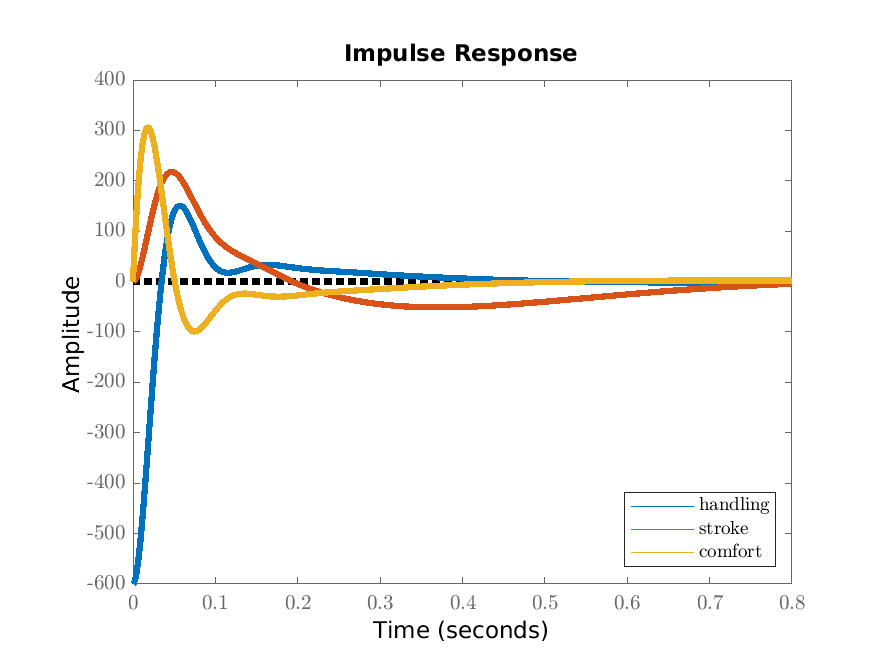
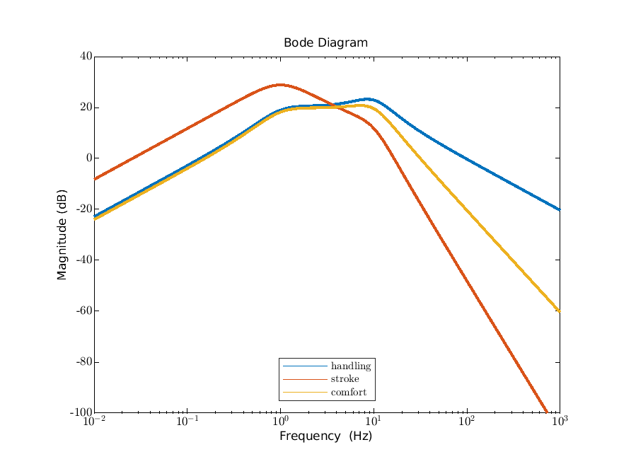
We give the impulse responses in Figure 15.1a and the Bode magnitude diagrams in Figure 15.1b. Comparing these to Figures 7.3 and 6.7, we see that the output is far less oscillatory and the peaks in the Bode diagram are far less pronounced.