Chapter 2 First order systems of differential equations
We consider input-state-output systems with a state \(x:[0,\infty )\to \mR ^n\), input \(u:[0,\infty )\to \mR ^{m}\) and output \(y:[0,\infty )\to \mR ^{p}\) described by
\(\seteqnumber{0}{2.}{0}\)\begin{equation} \label {eq:xy} \dot {x}=Ax+Bu,\qquad y=Cx+Du, \end{equation}
with the initial condition \(x(0)=x^0\) where \(x^0\in \mR ^n\) and
\[ A\in \mR ^{n\times n},~ B\in \mR ^{n\times m},~ C\in \mR ^{p\times n},~ D\in \mR ^{p\times m}. \]
-
Remark 2.1. For a given input \(u\) and initial condition \(x^0\), the solution \(x\) is unique and is given by (this is called the variation of parameters formula):
\[ x(t)=\e ^{At}x^0+\int _0^t \e ^{A(t-\theta )}Bu(\theta )\,d\theta , \]
where the matrix exponential function is given by
\[ \e ^{Az}=\sum _{k=0}^\infty \frac {1}{k!}A^kz^k. \]
The output is then given by
\(\seteqnumber{0}{2.}{1}\)\begin{equation} \label {eq:varpary} y(t)=C\e ^{At}x^0+\int _0^t C\e ^{A(t-\theta )}Bu(\theta )\,d\theta +Du(t). \end{equation}
-
Remark 2.2. Although the matrix exponential function is defined as a power series, the best way to calculate it is usually through eigenvalues and (generalized) eigenvectors of the matrix \(A\). See MA20220 Ordinary Differential Equations and Control.
Similarly, the variation of parameters formula is often not the easiest way to compute the solution.
-
Definition 2.3. For the input-state-output system (2.1) we define the following functions (here \(\sigma (A)\) denotes the set of eigenvalues of \(A\)):
-
• the step response \(H:[0,\infty )\phantom {]}\to \mR ^{p\times m}\) by \(H(t)=\int _0^t C\e ^{A\theta }B\,d\theta +D\);
-
• the impulse response \(h:[0,\infty )\phantom {]}\to \mR ^{p\times m}\) as the derivative of the step response;
-
• the transfer function \(G:\mC \backslash \sigma (A)\to \mC ^{p\times m}\) by \(G(s)=C(sI-A)^{-1}B+D\);
-
• the frequency response \(F:\mR \backslash i\sigma (A)\to \mC ^{p\times m}\) by \(F(\omega ):=G(i\omega )\).
-
-
Remark 2.4. Note that \(H\) and \(h\) are real-matrix-valued functions of a real variable, that \(G\) is a complex-matrix-valued function of a complex variable (and is undefined when \(s\) is an eigenvalue of \(A\)) and that \(F\) is a complex-matrix-valued function of a real variable (and is undefined when \(i\omega \) is an eigenvalue of \(A\))
-
Remark 2.5. When \(D=0\), the impulse response is given by \(h(t)=C\e ^{At}B\). More generally it is given by \(h=C\e ^{At}B+D\delta \) where \(\delta \) denotes the Dirac delta (at zero); we will not need the case \(D\neq 0\) though, so do not worry if you haven’t seen the Dirac delta before. From this and the variation of parameters formula (2.2) we see that when \(x^0=0\) we have
\[ y(t)=\int _0^t h(t-\theta )u(\theta )\,d\theta . \]
This should make clear the significance of the impulse response: from it we can determine the output for any input (when the initial condition is zero).
-
Remark 2.6. Each of the four functions in Definition 2.3 uniquely determines the other three. Combined with Remark 2.5, this shows that each of the four functions uniquely determines the output for any input (when the initial condition is zero).
-
• We can obtain the step response as the anti-derivative of the impulse response which is zero in zero (when \(D=0\)).
-
• We can obtain the transfer function as the Laplace transform of the impulse response (and therefore the impulse response as the inverse Laplace transform of the transfer function).
-
• We can obtain the transfer function from the frequency response since the transfer function is a rational function and it is therefore uniquely determined by its values on the imaginary axis.
We also have that the frequency response is the Fourier transform (the angular frequency non-unitary flavour) of the impulse response.
-
-
Remark 2.7. Although we have defined the four functions in Definition 2.3 using certain formulas, it is often easier to calculate them in a different way. For each of the four functions we have a separate chapter which in part deals with this.
2.1 Examples
-
Example 2.8. The scalar first order differential equation \(\dot {x}+x=u\) is of the form (2.1) with
\[ n=1,~~m=1,~~p=1,~~A=-1,~~B=1,~~C=1,~~D=0. \]
-
Example 2.9. The scalar second order differential equation \(\ddot {q}+2\zeta \dot {q}+q=u\), \(y=q\) is of the form (2.1) with
\[ x=\bbm {q\\\dot {q}},~~n=2,~~m=1,~~p=1,~~A=\bbm {0&1\\-1&-2\zeta },~~B=\bbm {0\\1},~~C=\bbm {1&0},~~D=0. \]
Note that if we write \(\dot {x}=Ax+Bu\) in components, we obtain
\[ \dot {x}_1=x_2,\qquad \dot {x}_2=-x_1-2\zeta x_2+u. \]
Substituting the first equation into the second gives
\[ \dot {x}_1=x_2,\qquad \ddot {x}_1=-x_1-2\zeta \dot {x}_1+u. \]
With \(q:=x_1\) the second equation now indeed is \(\ddot {q}+2\zeta \dot {q}+q=u\) and the first equation tells us that \(x_2=\dot {q}\).
2.2 Cases studies*
For the case studies (and in later chapters) we consider the slightly more general situation of an input-state-output system with two inputs and two outputs.
We consider input-state-output systems with a state \(x:[0,\infty )\to \mR ^n\), external input \(w:[0,\infty )\to \mR ^{m_1}\), control input \(u:[0,\infty )\to \mR ^{m_2}\), performance output \(z:[0,\infty )\to \mR ^{p_1}\) and measured output \(y:[0,\infty )\to \mR ^{p_2}\) described by
\(\seteqnumber{0}{2.}{2}\)\begin{equation} \label {eq:xzy} \dot {x}=Ax+B_1w+B_2u,\qquad z=C_1x+D_{11}w+D_{12}u,\qquad y=C_2x+D_{21}w+D_{22}u, \end{equation}
with the initial condition \(x(0)=x^0\) where \(x^0\in \mR ^n\) and
\(\seteqnumber{0}{2.}{3}\)\begin{gather} \label {eq:ABCDmatrices} A\in \mR ^{n\times n},~ B_1\in \mR ^{n\times m_1},~ B_2\in \mR ^{n\times m_2},\notag \\ C_1\in \mR ^{p_1\times n},~ D_{11}\in \mR ^{p_1\times m_1},~ D_{12}\in \mR ^{p_1\times m_2},~ C_2\in \mR ^{p_2\times n},~ D_{21}\in \mR ^{p_2\times m_1}, D_{22}\in \mR ^{p_2\times m_2}. \end{gather}
2.2.1 Case study: control of a tape drive
Most data in the world is not stored on hard drives, but on tape drives. See Figure 2.1 for a photo of a tape drive. The tape drive contains two reels which rotate due to currents being applied to motors. This causes the tape to be transported from one reel (the supply reel) to the other reel (the take-up reel). In between the reels is the read/write head. The objectives are for the velocity at the read/write head to be some given constant and for the tension in the tape to be some given constant (both are needed for the read/write operation to be performed well).
We initially model this situation assuming that the reels (including the tape wrapped around it) is perfectly circular. This however is not strictly true. To account for this, we include a disturbance. Since we have a rotational system, it is natural to assume that this disturbance is periodic with a known period.
The rationale here is similar to what is done in statistical modeling where there usually is a model “plus noise”. Here however we assume that the additional term is deterministic and instead of assuming some statistical properties of this term (such as it being Gaussian with known mean and variance), we assume that we know that it is periodic with a known period.

A simple model for the tape drive is:
\(\seteqnumber{0}{2.}{4}\)\begin{align*} M_1\dot {v}_1+d_1v_1-T&=u_1,\\ M_2\dot {v}_2+d_2v_2+T&=u_2,\\ \dot {T}+k(v_1-v_2)&=kv_e. \end{align*} Here \(v_1\) is the linear velocity at the supply reel (and the head), \(v_2\) is the linear velocity at the take-up reel, \(T\) is the tension in the tape, \(u_1\) and \(u_2\) are the controls and \(v_e\) is the periodic disturbance (with frequency \(\omega _e\)). The parameters are \(M_1,M_2,d_1,d_2,k>0\). We denote the desired velocity at the read/write head by \(r_v\) and the desired tension in the tape by \(r_T\) (here the letter \(r\) standard for “reference”). We assume that we can measure both velocities and the tension and that we know the desired velocity \(r_v\) and tension \(r_T\).
If we need to consider specific parameter values, then we make the choice
\[ M_1=0.25,\quad M_2=0.15,\quad d_1=1,\quad d_2=1,\quad k=170,\quad r_v=5,\quad r_T=0.3,\quad \omega _e=650. \]
We can write this model in the standard state space form (2.3) with
\[ x:=\bbm {v_1\\v_2\\T},\qquad w=\bbm {r_v\\r_T\\v_e},\qquad u=\bbm {u_1\\u_2},\qquad z=\bbm {v_1-r_v\\T-r_T},\qquad y=\bbm {v_1\\v_2\\T\\r_v\\r_T}, \]
(i.e. \(z_1\) is the difference between the velocity at the head and its reference and \(z_2\) is the difference between the tension in the tape and its reference) and
\(\seteqnumber{0}{2.}{4}\)\begin{gather*} A=\bbm { -\frac {d_1}{M_1}&0&\frac {1}{M_1}\\ 0&-\frac {d_2}{M_2}&-\frac {1}{M_2}\\ -k&k&0 },\qquad B_1=\bbm {0&0&0\\0&0&0\\0&0&k},\qquad B_2=\bbm {\frac {1}{M_1}&0\\0&\frac {1}{M_2}\\0&0}, \\ C_1=\bbm {1&0&0\\0&0&1},\qquad D_{11}=\bbm {-1&0&0\\0&-1&0}, \\ C_2=\bbm { 1&0&0\\ 0&1&0\\ 0&0&1\\ 0&0&0\\ 0&0&0 },\qquad D_{21}=\bbm { 0&0&0\\ 0&0&0\\ 0&0&0\\ 1&0&0\\ 0&1&0 }. \end{gather*}
2.2.2 Case study: a suspension system
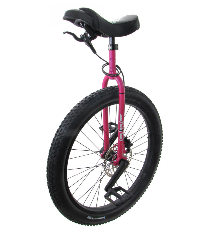
We consider what in the automotive industry is called a quarter-car model. This is used as a first step in designing suspension systems for cars. The quarter-car model considers only one wheel (and therefore ignores the motion of the car due to coupling of the wheels). Therefore, we might also think of designing a syspension system for a unicycle (Figure 2.2).

The vertical position, velocity and acceleration of the car are considered (since this is relevant for the suspension system). The road profile (curbs, speed bumps, potholes, general roughness of the road) is an external input. This road profile is given as a vertical position as a function of horizontal position. If we assume the car moves at constant horizontal velocity, then we can view the road profile as a function of time instead. In our modelling we will consider the derivative of this road profile with respect to time, the road velocity, as the (external) input.
We model the tyre as a spring and we include a mass for the part of the car below the suspension system (this includes the tyre, the wheel and so on). In the automotive industry these are called the unsprung spring and unsprung mass. The main part of the car (the part above the suspension system) is modelled as a mass, called the sprung mass.
The suspension system is between the two masses. We have the following differential equations:
\(\seteqnumber{0}{2.}{4}\)\begin{gather*} m_s\dot {v}_s+F_u=0,\qquad m_{us}\dot {v}_{us}+F_{us}-F_u=0,\\ \dot {q}=v_{us}-v_s,\qquad \dot {F}_{us}=k_{us}(v_{us}-v_e). \end{gather*} Here \(v_s\) is the velocity of the sprung mass, \(v_{us}\) is the velocity of the unsprung mass, \(F_{us}\) is the force across the unsprung spring (i.e. the tyre) and \(q\) is the distance between the two masses plus a constant (we normalize that constant so that \(q=0\) gives the “desired” distance between the masses). The constants are \(m_s>0\) (the sprung mass), \(m_{us}>0\) (the unsprung mass) and \(k_{us}>0\) (the stiffness of the unsprung spring, i.e. the tyre). The external input \(v_e\) is the road velocity (as described above) and \(F_u\) is the force applied by the suspension system (i.e. \(F_u\) is what we have to design).
We can write this model in the standard state space form (2.3) with
\[ x:=\bbm {F_{us}\\v_{us}\\q\\v_s},\qquad w:=v_e,\qquad u:=F_u, \]
and
\[ A=\bbm {0&k_{us}&0&0\\ \frac {-1}{m_{us}}&0&0&0\\ 0&1&0&-1\\ 0&0&0&0 },\qquad B_1=\bbm {-k_{us}\\0\\0\\0},\qquad B_2=\bbm {0\\\frac {1}{m_{us}}\\0\\\frac {-1}{m_s}}. \]
There are three variables relevant for the performance output:
-
• The tyre deflection \(\int v_{us}-v_e\), which is a measure for handling.
-
• The suspension stroke \(q\), which shouldn’t be too large in absolute value as this would damage the car (\(q\ll 0\) means that the masses get too close and might collide, \(q\gg 0\) means that the masses are too far apart so that the suspension system gets too streched).
-
• The acceleration of the sprung mass, \(\dot {v}_{s}\), which is a measure for comfort.
In terms of the state variables and the control (using the differential equations) we have that the tyre deflection is \(\frac {x_1}{k_{us}}\), the suspension stroke is \(x_3\) and the acceleration of the sprung mass equals \(\frac {-u}{m_s}\). We want all three of these quantities to be small. Which one we care about most depends on the application (for a formula one car, we would mostly be interested in tyre deflection whereas for a normal car we would relatively speaking care more about the acceleration of the sprung mass). To take this into account, we introduce weights \(r_1,r_2>0\) and define the performance output by
\[ z=\bbm {r_1\frac {x_1}{k_{us}}\\r_2x_3\\\frac {-u}{m_s}}. \]
In standard form this gives
\[ C_1=\bbm {\frac {r_1}{k_{us}}&0&0&0\\0&0&r_2&0\\0&0&0&0},\qquad D_{12}=\bbm {0\\0\\\frac {-1}{m_s}}. \]
If we need to consider specific parameter values, then we make the choice
\[ m_s=250,\quad m_{us}=35,\quad k_{us}=150,\!000,\quad r_1=\frac {k_{us}}{m_s},\quad r_2=r_1\sqrt {\frac {m_{us}}{m_s}}. \]
In principle it is possible to measure the whole state, but this comes at a cost. Easy measurements are \(q\) and \(v_{us}-v_s\) and a suspension system which uses only knowledge of these two variables is easier to physically build. In either case we need to add measurement noise/unmodelled dynamics. This gives (when measuring the whole state)
\[ \qquad C_2=I,\qquad D_{21}=\bbm {0&\delta _1&0&0&0\\0&0&\delta _2&0&0\\0&0&0&\delta _3&0\\0&0&0&0&\delta _4\\},\qquad \]
or (when measuring only \(q\) and \(v_{us}-v_s\))
\[ C_2=\bbm {0&0&1&0\\0&1&0&-1}, \qquad D_{21}=\bbm {0&\delta _1&0\\0&0&\delta _2}, \]
where \(\delta _1,\delta _2,\delta _3,\delta _4>0\). In both cases, we need to write \(v_e=w_1\) and change \(B_1\) accordingly (by adding zero columns).
Our ultimate aim is to design an “optimal” suspension system. However to understand the issues better, we will also consider a suspension system consisting of a spring and a damper between the two masses. This gives (here \(k_s,d>0\))
\[ u=d(v_s-v_{us})-k_sq,\qquad \text {i.e.,}~~u=d(x_4-x_2)-k_sx_3. \]
We then obtain the closed-loop system (here we ignore the measured output \(y\) and therefore just have \(w=v_e\))
\[ \dot {x}=A_\cl x+B_\cl w,\qquad z=C_\cl x, \]
with
\[ A_\cl =\bbm {0&k_{us}&0&0\\ \frac {-1}{m_{us}}&\frac {-d}{m_{us}}&\frac {-k_s}{m_{us}}&\frac {d}{m_{us}}\\ 0&1&0&-1\\ 0&\frac {d}{m_s}&\frac {k_s}{m_s}&\frac {-d}{m_s} },\qquad B_\cl =\bbm {-k_{us}\\0\\0\\0},\qquad C_\cl =\bbm {\frac {r_1}{k_{us}}&0&0&0\\ 0&0&r_2&0\\ 0&\frac {d}{m_s}&\frac {k_s}{m_s}&\frac {-d}{m_s} }. \]
This closed-loop system describes how our performance output \(z\) depends on the external input \(w\) (here the road velocity) when we choose the control input (i.e. the suspension system) \(u\) as above.
For illustrative purposes we will also consider non-optimal (but reasonable) values for \(k_s\) and \(d\); these we pick as
\[ k_s=50,\!000,\qquad d=k_s~\sqrt {\frac {m_s+m_{us}}{k_{us}}}. \]