Chapter 11 Output regulation and disturbance rejection: the measurement feedback case
We consider input-state-output systems with a state \(x:[0,\infty )\to \mR ^n\), external input \(w:[0,\infty )\to \mR ^{m_1}\), control input \(u:[0,\infty )\to \mR ^{m_2}\), performance output \(z:[0,\infty )\to \mR ^{p_1}\) and measured output \(y:[0,\infty )\to \mR ^{p_2}\) described by
\(\seteqnumber{0}{11.}{0}\)\begin{equation} \label {eq:OR:xzy} \dot {x}=Ax+B_1w+B_2u,\qquad z=C_1x+D_{11}w,\qquad y=C_2x+D_{21}w, \end{equation}
with the initial condition \(x(0)=x^0\) where \(x^0\in \mR ^n\) and
\[ A\in \mR ^{n\times n},~ B_1\in \mR ^{n\times m_1},~ B_2\in \mR ^{n\times m_2},~ C_1\in \mR ^{p_1\times n},~ D_{11}\in \mR ^{p_1\times m_1},~ C_2\in \mR ^{p_2\times n},~ D_{21}\in \mR ^{p_2\times m_1}. \]
We assume that the external input \(w\) is generated by an exo-system
\[ \dot {x}_e=A_ex_e,\qquad w=C_ex_e, \]
with the initial condition \(x_e(0)=x_e^0\) where \(x_e^0\in \mR ^{n_e}\) and
\[ A_e\in \mR ^{n_e\times n_e},\qquad C_e\in \mR ^{m_1\times n_e}. \]
-
Definition 11.1 (Measurement feedback output regulation and disturbance rejection problem). The objective is to find matrices
\[ A_c\in \mR ^{n_c\times n_c},~ B_c\in \mR ^{n_c\times p_2},~ C_c\in \mR ^{m_2\times n_c},~ D_c\in \mR ^{m_2\times p_2}, \]
such that with the control
\(\seteqnumber{0}{11.}{1}\)\begin{equation} \label {eq:OR:controller} \dot {x}_c=A_cx_c+B_cy,\quad u=C_cx_c+D_cy, \end{equation}
where \(x_c(0)=x_c^0\), the following two conditions are both satisfied:
-
1. for all \(x^0\), \(x_c^0\) and \(x_e^0\) we have \(\lim _{t\to \infty }z(t)=0\);
-
2. for \(x_e^0=0\) and all \(x^0\) and \(x_c^0\) we have \(\lim _{t\to \infty }x(t)=0\) and \(\lim _{t\to \infty }x_c(t)=0\).
The first of these is the regulation requirement, the second is the stability requirement.
-
-
Theorem 11.3. Assume that \((A,B_2)\) is stabilizable, that \(\left (\sbm {A&B_1C_e\\0&A_e},\bbm {C_2&D_{21}C_e}\right )\) is detectable and that the regulator equations have a solution \(\Pi \), \(V\). Let \(F_1\in \mR ^{m_2\times n}\) be such that \(A+B_2F_1\) is asymptotically stable and let \(L\in \mR ^{(n+n_e)\times p_2}\) be such that \(\sbm {A&B_1C_e\\0&A_e}-L\bbm {C_2&D_{21}C_e}\) is asymptotically stable. Then
\(\seteqnumber{0}{11.}{2}\)\begin{gather*} A_c=\bbm {A&B_1C_e\\0&A_e}-L\bbm {C_2&D_{21}C_e}+\bbm {B_2\\0}\bbm {F_1&V-F_1\Pi },\\ B_c=L,\qquad C_c=\bbm {F_1&V-F_1\Pi },\qquad D_c=0, \end{gather*} solves the measurement feedback output regulation and disturbance rejection problem.
Moreover, for all \(x^0\), \(x_c^0\) and \(x_e^0\) we have \(\lim _{t\to \infty } x(t)-\Pi x_e(t)=0\).
-
Remark 11.4. If \(D_c=0\), then we can write the combination of (11.1) and (11.2) as
\[ \bbm {\dot {x}\\\dot {x}_c}=\bbm {A&B_2C_c\\B_cC_2&A_c}\bbm {x\\x_c}+\bbm {B_1\\B_cD_{21}}w,\qquad z=\bbm {C_1&0}\bbm {x\\x_c}+D_{11}w, \]
which we can view as an input/state/output system with input \(w\) and output \(z\).
If \(D_c\neq 0\), then the formulas become more complicated. We do not need that case.
11.1 Examples
-
Example 11.5. Consider the first order scalar differential equation
\[ \dot {x}+x=w+u. \]
The objective is to find a control \(u\) such that \(\lim _{t\to \infty }x(t)=0\) no matter what \(x(0)\) is when \(w(t)=d\) where \(d\in \mR \) is unknown. Assume that \(y=x\) is the measurement.
This is of the standard form with
\[ A=-1,\quad B_1=1,\quad B_2=1,\quad C_1=1,\quad D_{11}=0,\quad C_2=1,\quad D_{21}=0, \]
and (so that \(w=x_e=x_e^0=d\))
\[ A_e=0,\qquad C_e=1. \]
The regulator equations are
\[ -\Pi +1+V=0,\qquad \Pi =0, \]
which gives \(\Pi =0\), \(V=-1\). Since \(A\) is stable, we can take \(F_1=0\). In the full-information case, this would give \(u=-d\) as control (which cancels the disturbance \(w\) completely); however, here we assume that \(u\) can only depend on the measurement \(y=x\) (and therefore not directly on \(d\)).
We have
\[ \bbm {A&B_1C_e\\0&A_e}-\bbm {L_1\\L_2}\bbm {C_1&D_{21}C_e}= \bbm {-1&1\\0&0}-\bbm {L_1\\L_2}\bbm {1&0} =\bbm {-1-L_1&1\\-L_2&0}. \]
The characteristic polynomial of this matrix is \(s^2+(1+L_1)s+L_2\), which is stable if and only if \(1+L_1>0\) and \(L_2>0\). We can therefore choose \(L_1=0\) and \(L_2=1\). We see that the detectability condition from Theorem 11.3 is satisfied. The controller from that theorem is
\[ A_c=\bbm {-1&0\\-1&0},\quad B_c=\bbm {0\\1},\quad C_c=\bbm {0&-1},\quad D_c=0. \]
Theorem 11.3 tells us that this solves our problem, but to see this more explicitly, we investigate further. The differential equations for the controller are
\[ \dot {x}_{c,1}=-x_{c,1},\quad \dot {x}_{c,2}=x-x_{c,1},\quad u=-x_{c,2}. \]
From this we can get a differential equation for the control \(u\)
\[ \ddot {u}+\dot {u}+u=-d, \]
since
\[ \ddot {u}+\dot {u}+u=-\ddot {x}_{c,2}-\dot {x}_{c,2}+u =-(\dot {x}-\dot {x}_{c,1})-(x-x_{c,1})+u=-\dot {x}-x+u=-d. \]
From this we see that \(u\) equals \(-d\) plus a term which decays to zero; so “asymptotically” we get back the full-information control \(-d\).
-
Remark 11.6. In Example 11.5 we can pick an appropriate \(L\) using Routh–Hurwitz. This is however for the very simple case \(n=n_e=1\). For larger \(n\) and/or \(n_e\) this becomes very tedious. Therefore we would like simple necessary and sufficient conditions for detectability. We will obtain those in Chapter 16.
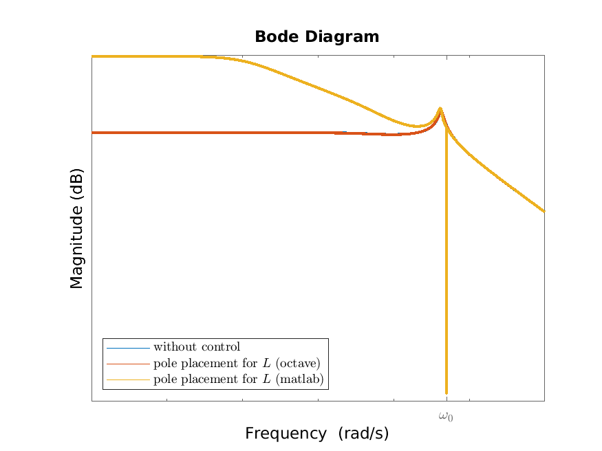
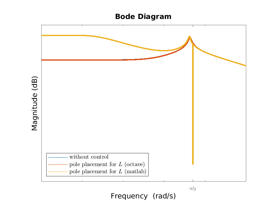
11.2 Case study: control of a tape drive*
We consider the measurement feedback output regulation and disturbance rejection problem for the tape drive system. In addition to what we did for the full information feedback problem in Section 9.2, we need to find an output injection matrix \(L\) which makes \(\sbm {A&B_1C_e\\0&A_e}-L\bbm {C_2&D_{21}C_e}\) asymptotically stable. As this is a 7-by-3 matrix, this is non-trivial to do by hand. Therefore, we do this numerically using eigenvalue placement. The eigenvalues of \(\sbm {A&B_1C_e\\0&A_e}\) are the union of those of \(A\), which are stable by Section 3.3 and which we want to leave as they are, and those of \(A_e\), which are \(0\) (with multiplity 2) and \(\pm i\omega _e\), which are unstable and which we want to move slightly to the left. The resulting Bode magnitude plots from \(v_e\) to \(v_1-r_v\) and \(T-r_T\) are given in Figure 11.1 (and are compared to those without any control). We can clearly see the effect of the disturbance rejection at the frequency \(\omega _0\). The choice of the desired characteristic polynomial does not uniquely determine the matrix \(L\) (this is because \(p_2>1\)). The algorithms utilized by matlab and octave produce different \(L\)’s with the one produced by octave being clearly superior (though both achieve the given objective).