Chapter 20 \(H^2\) control: the state feedback case
We consider input-state-output systems with a state \(x:[0,\infty )\to \mR ^n\), external input \(w:[0,\infty )\to \mR ^{m_1}\), control input \(u:[0,\infty )\to \mR ^{m_2}\) and performance output \(z:[0,\infty )\to \mR ^{p_1}\) described by
\(\seteqnumber{0}{20.}{0}\)\begin{equation} \label {eq:H2:xz} \dot {x}=Ax+B_1w+B_2u,\qquad z=C_1x+D_{12}u, \end{equation}
with the initial condition \(x(0)=x^0\) where \(x^0\in \mR ^n\) and
\(\seteqnumber{0}{20.}{1}\)\begin{equation} \label {eq:control:xzmatrices} A\in \mR ^{n\times n},~ B_1\in \mR ^{n\times m_1},~ B_2\in \mR ^{n\times m_2},~ C_1\in \mR ^{p_1\times n},~ D_{12}\in \mR ^{p_1\times m_2}. \end{equation}
-
Definition 20.1 (\(H^2\) state feedback problem). The objective is to find a matrix
\[ F\in \mR ^{m_2\times n}, \]
such that with the control \(u=Fx\) the following two conditions are both satisfied
-
1. \(\int _{-\infty }^\infty \|F_{zw}(\omega )\|_{\HS }^2\,d\omega \) is minimized amongst all such \(F\),
-
2. for all \(x^0\) and \(w=0\) we have \(\lim _{t\to \infty }x(t)=0\),
where \(F_{zw}\) is the frequency response of the closed-loop system
\(\seteqnumber{0}{20.}{2}\)\begin{equation} \label {eq:closedH2} \dot {x}=(A+B_2F)x+B_1w,\qquad z=(C_1+D_{12}F)x. \end{equation}
-
-
Remark 20.3. By Plancherel’s equality we have
\[ \frac {1}{2\pi }\int _{-\infty }^\infty \|F_{zw}(\omega )\|_{\HS }^2\,d\omega =\int _0^\infty \|h_{zw}(t)\|_{\HS }^2\,dt, \]
where \(h_{zw}\) is the impulse response, so that equivalently to (1) in Definition 20.1 we could have:
-
• \(\int _0^\infty \|h_{zw}(t)\|_{\HS }^2\,dt\) is minimized amongst all such \(F\), where \(h_{zw}\) is the impulse response of the closed-loop system (20.3)
-
-
Theorem 20.4. Assume that \(D_{12}\) is injective, that \((A,B_2)\) is stabilizable and that the Rosenbrock matrix
\[ \bbm {sI-A&-B_2\\C_1&D_{12}}, \]
is injective for all \(s\in \mC \) with \(\re (s)=0\). Then there exists a unique solution \(X\) of the algebraic Riccati equation
\(\seteqnumber{0}{20.}{3}\)\begin{equation} \label {eq:RiccatiH2} A^*X+XA+C_1^*C_1-(XB_2+C_1^*D_{12})(D_{12}^*D_{12})^{-1}(B_2^*X+D_{12}^*C_1)=0, \end{equation}
such that \(A+B_2F\) is asymptotically stable where
\[ F=-(D_{12}^*D_{12})^{-1}\left (D_{12}^*C_1+B_2^*X\right ). \]
This \(X\) is symmetric positive semidefinite. Furthermore, \(F\) is the unique solution of the \(H^2\) state feedback problem and
\[ \trace (B_1^*XB_1) =\frac {1}{2\pi }\int _{-\infty }^\infty \|F_{zw}(\omega )\|_{\HS }^2\,d\omega =\int _0^\infty \|h_{zw}(t)\|_{\HS }^2\,dt. \]
-
Remark 20.6. Definition 20.1 and Theorem 20.4 consider the \(H^2\) state feedback problem with stability; similarly as in Chapter 18, the \(H^2\) state feedback problem without stability can be formulated and solved: this involves the smallest symmetric positive semidefinite solution of the algebraic Riccati equation (it can be shown that the stabilizing solution from Theorem 20.4 is the largest symmetric positive semidefinite solution) and does not involve the stabilizability and Rosenbrock conditions.
20.1 Examples
-
Example 20.7. Consider the first order scalar differential equation
\[ \dot {x}(t)+x(t)=w(t)+u(t). \]
For the \(H^2\) state feedback problem, we consider the performance output
\[ z(t)=\bbm {x(t)\\\varepsilon u(t)}, \]
where \(\varepsilon >0\). To put this into the \(H^2\) state feedback framework, we have \(n=m_1=m_2=1\), \(p_1=2\) and
\[ A=-1,\quad B_1=1,\quad B_2=1,\quad C_1=\bbm {1\\0},\quad D_{12}=\bbm {0\\\varepsilon }. \]
The Riccati equation is the same as in Example 18.5, so that
\[ X=-\varepsilon ^2+\varepsilon \sqrt {\varepsilon ^2+1}, \qquad F=1-\sqrt {1+\varepsilon ^{-2}}. \]
-
Example 20.8. Consider the undamped second order scalar differential equation
\[ \ddot {q}(t)+q(t)=w(t)+u(t), \]
with the state \(x=\sbm {q\\\dot {q}}\) and the performance output
\[ z=\bbm {\dot {q}\\\varepsilon u}, \]
where \(\varepsilon >0\). To put this into the \(H^2\) state feedback framework, we have \(n=2\), \(m_1=m_2=1\), \(p_1=2\) and
\[ A=\bbm {0&1\\-1&0},\quad B_1=\bbm {0\\1},\quad B_2=\bbm {0\\1},\quad C_1=\bbm {0&1\\0&0},\qquad D_{12}=\bbm {0\\\varepsilon }, \]
The Riccati equation is the same as in Example 19.1, so that
\[ X=\varepsilon \bbm {1&0\\0&1},\qquad F=\bbm {0&-\varepsilon ^{-1}}. \]
20.2 Case study: a suspension system*
We consider the state feedback \(H^2\) problem for the suspension system design. By Section 13.3, the system is controllable and therefore stabilizable. We clearly have that \(D_{12}\) is injective. We now consider the Rosenbrock condition from Theorem 20.4.
The Rosenbrock matrix is
\[ \bbm {sI-A&-B_2\\C_1&D_{12}}= \bbm { s&-k_{us}&0&0&0\\ \frac {1}{m_{us}}&s&0&0&\frac {-1}{m_{us}}\\ 0&-1&s&1&0\\ 0&0&0&s&\frac {1}{m_s}\\ \frac {r_1}{k_{us}}&0&0&0&0\\ 0&0&r_2&0&0\\ 0&0&0&0&\frac {-1}{m_s} }. \]
To show that this is injective, we need to identify 5 independent rows; we pick rows 1,3,5,6 and 7. That gives the submatrix
\[ \bbm { s&-k_{us}&0&0&0\\ 0&-1&s&1&0\\ \frac {r_1}{k_{us}}&0&0&0&0\\ 0&0&r_2&0&0\\ 0&0&0&0&\frac {-1}{m_s} }. \]
To show that this is indeed injective, we calculate its determinant. We develop by the last row to obtain
\[ \frac {-1}{m_s}\det \bbm { s&-k_{us}&0&0\\ 0&-1&s&1\\ \frac {r_1}{k_{us}}&0&0&0\\ 0&0&r_2&0\\ }, \]
we develop this by the last column to obtain
\[ \frac {-1}{m_s}\det \bbm { s&-k_{us}&0\\ \frac {r_1}{k_{us}}&0&0\\ 0&0&r_2\\ }, \]
developing this by the last row gives
\[ \frac {-r_2}{m_s}\det \bbm { s&-k_{us}\\ \frac {r_1}{k_{us}}&0\\ }=\frac {-r_1r_2}{m_s}, \]
which is nonzero when \(r_1,r_2>0\).
We investigate what happens when \(r_1\) or \(r_2\) equals zero. If \(r_2=0\), then when \(s=0\) the third column of the Rosenbrock matrix equals zero; therefore the Rosenbrock condition does not hold. If \(r_1=0\), then we consider rows 1,3,4,6 and 7 of the Rosenbrock matrix:
\[ \bbm { s&-k_{us}&0&0&0\\ 0&-1&s&1&0\\ 0&0&0&s&\frac {1}{m_s}\\ 0&0&r_2&0&0\\ 0&0&0&0&\frac {-1}{m_s} }, \]
whose determinant we develop by the last row to obtain
\[ \frac {-1}{m_s} \det \bbm { s&-k_{us}&0&0\\ 0&-1&s&1\\ 0&0&0&s\\ 0&0&r_2&0\\ }, \]
and develop by the last row to obtain
\[ \frac {r_2}{m_s} \det \bbm { s&-k_{us}&0\\ 0&-1&1\\ 0&0&s\\ }, \]
and since this matrix is upper triangular, this equals
\[ \frac {-s^2r_2}{m_s}. \]
Therefore, as long as \(s\neq 0\), these rows are linearly independent. If \(s=0\), then we instead consider rows 1,2,3,6 and 7 and obtain
\[ \bbm { 0&-k_{us}&0&0&0\\ \frac {1}{m_{us}}&0&0&0&\frac {-1}{m_{us}}\\ 0&-1&0&1&0\\ 0&0&r_2&0&0\\ 0&0&0&0&\frac {-1}{m_s} }. \]
Developing the determinant by the last row gives
\[ \frac {-1}{m_s}\det \bbm { 0&-k_{us}&0&0\\ \frac {1}{m_{us}}&0&0&0\\ 0&-1&0&1\\ 0&0&r_2&0 }, \]
developing by the last row again gives
\[ \frac {r_2}{m_s}\det \bbm { 0&-k_{us}&0\\ \frac {1}{m_{us}}&0&0\\ 0&-1&1 }, \]
developing by the last column gives
\[ \frac {r_2}{m_s}\det \bbm { 0&-k_{us}\\ \frac {1}{m_{us}}&0 }=\frac {r_2k_{us}}{m_sm_{us}}. \]
Therefore, for \(s=0\), these rows are linearly independent. So if \(r_1=0\), then the Rosenbrock condition is still satisfied. Therefore the suspension stroke term needs to be present in the cost function for the Rosenbrock condition to be satisfied, but the tyre deflection (“handling”) term could be absent and the conditions from Theorem 20.4 would still be satisfied.
The algebraic Riccati equation is too complicated to solve by hand. We use the specific parameter values from the introduction to solve it numerically. This gives the state feedback matrix
\[ F=\bbm {-0.2944&-1908&-56125&6027}. \]
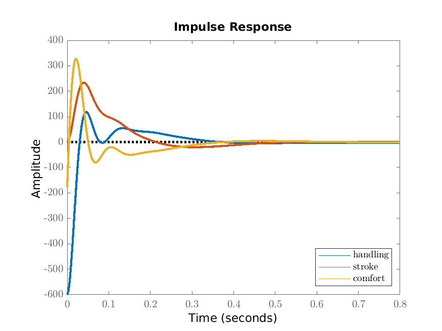
We give the impulse responses in Figure 20.1a and the Bode diagrams in Figure 20.1b. Comparing these to Figures 15.1a and 15.1b (the optimal fixed structure), we see that the output is less oscillatory and the peaks in the Bode diagram are slightly less pronounced.