Chapter 6 The frequency response
Recall that the frequency response of \(\dot {x}=Ax+Bu\), \(y=Cx+Du\) is given by \(F(\omega )=C(i\omega I-A)^{-1}B+D\).
-
Remark 6.2. We give an interpretation of the frequency response. We start with the case \(m=p=1\). We claim that with \(s\) not an eigenvalue of \(A\) for input \(u(t)=\e ^{st}\), a particular solution is given by \(x(t)=(sI-A)^{-1}B\e ^{st}\). We verify this by substitution: we have \(\dot {x}=s(sI-A)^{-1}B\e ^{st}\) and on the other hand we have
\[ Ax+Bu=A(sI-A)^{-1}B\e ^{st}+B\e ^{st}=\left [A+(sI-A)\right ](sI-A)^{-1}B\e ^{st}, \]
which also equals \(s(sI-A)^{-1}B\e ^{st}\). The corresponding output equals \(y(t)=\left [C(sI-A)^{-1}B+D\right ]\e ^{st}\). Putting \(s=i\omega \) we obtain \(y(t)=F(\omega )\e ^{i\omega t}\). Writing \(F(\omega )\) in polar coordinates gives \(F(\omega )=|F(\omega )|\e ^{i\arg (F(\omega ))}\) and therefore
\[ y(t)=|F(\omega )|\e ^{i(\omega t+\arg (F(\omega )))}. \]
Hence the particular output for input \(\e ^{i\omega t}\) equals \(|F(\omega )|\e ^{i(\omega t+\arg (F(\omega )))}\). Because the coefficient matrices \(A\), \(B\), \(C\) and \(D\) are real, taking the imaginary parts of this input gives the imaginary part of this corresponding output. Therefore a particular output for input \(\sin (\omega t)\) equals
\[ y(t)=|F(\omega )|\sin (\omega t+\arg (F(\omega ))). \]
This is only a particular solution, to obtain the general solution we would need to add the general solution of the homogeneous equation \(\dot {x}=Ax\), \(y=Cx\). However, if \(A\) is stable, then that general solution of the homogeneous equation will be “small” for “large” times and therefore we will mostly see the above particular solution. Hence to good approximation, the output for a sinusoid with frequency \(\omega \) is a sinusoid with the same frequency shifted by \(\arg (F(\omega ))\) and multiplied by \(|F(\omega )|\).
In the case \(m,p>1\) we apply the above componentwise. So if \(m=2\), then we first consider \(u_1=\sin (\omega t)\) and \(u_2=0\). If \(p=2\) we further first only consider \(y_1\) and conclude that a particular solution is of the form \(y_1(t)=|F_{11}(\omega )|\sin (\omega t+\arg (F_{11}(\omega )))\). By considering other combinations, we get similar interpretations of \(F_{12}\), \(F_{21}\) and \(F_{22}\) (in case \(m=p=2\)).
6.1 Examples
-
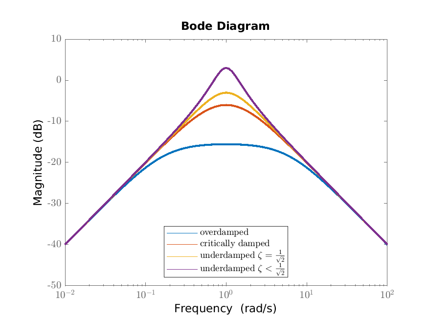
Example 6.4. The frequency response of the second order scalar differential equation
\[ \ddot {q}(t)+2\zeta \dot {q}(t)+q(t)=u(t),\quad y=q, \]
is
\[ F(\omega )=\frac {1}{-\omega ^2+2\zeta i\omega +1}. \]
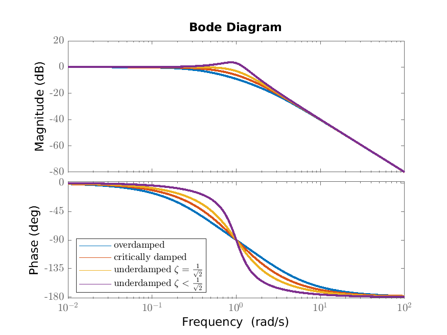
When \(\zeta \in [0,\frac {1}{\sqrt {2}})\phantom {]}\), \(|F(\omega )|\) has a maximum at \(\omega _{\rm max}:=\sqrt {1-2\zeta ^2}\). Instead, when \(\zeta \geq \frac {1}{\sqrt {2}}\), \(|F(\omega )|\) is monotonically decreasing (for \(\omega >0\)). So whereas \(\zeta =1\) is the value for which a qualitative difference in the step response occurs, it is for \(\zeta =\frac {1}{\sqrt {2}}\) that a qualitative difference in the frequency response occurs. In the problems you are asked to show this.
6.2 Figures*
-
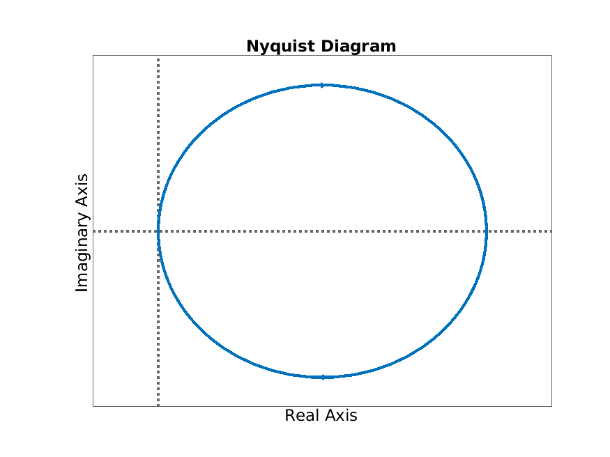
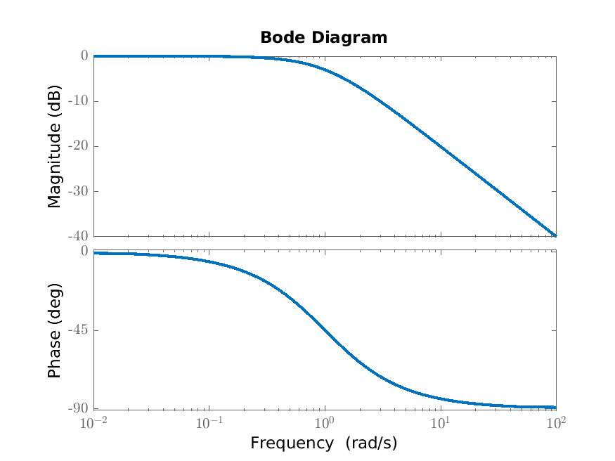
Remark 6.6. Since the frequency response is a complex-valued function of a real variable, it is not straightforward to plot (unlike for example the step response, which is a real-valued function of a real variable). There are essentially two common ways to plot it. The first is to treat \(\omega \) as a parameter and plot the curve \(\omega \mapsto F(\omega )\) in the complex plane; this is called the Nyquist diagram. The second is to plot \(|F(\omega )|\) and \(\arg (F(\omega ))\) separately as functions of \(\omega \) (since these are real-valued functions of a real variable, this is straightforward); it is common to use a logarithmic scale for \(\omega \) in both plots and in the magnitude plot to use a logarithmic scale on both axes; the combination of these plots are called the Bode diagram and separately they are called the Bode magnitude diagram and the Bode phase diagram. We will mainly be interested in the Bode magnitude diagram.
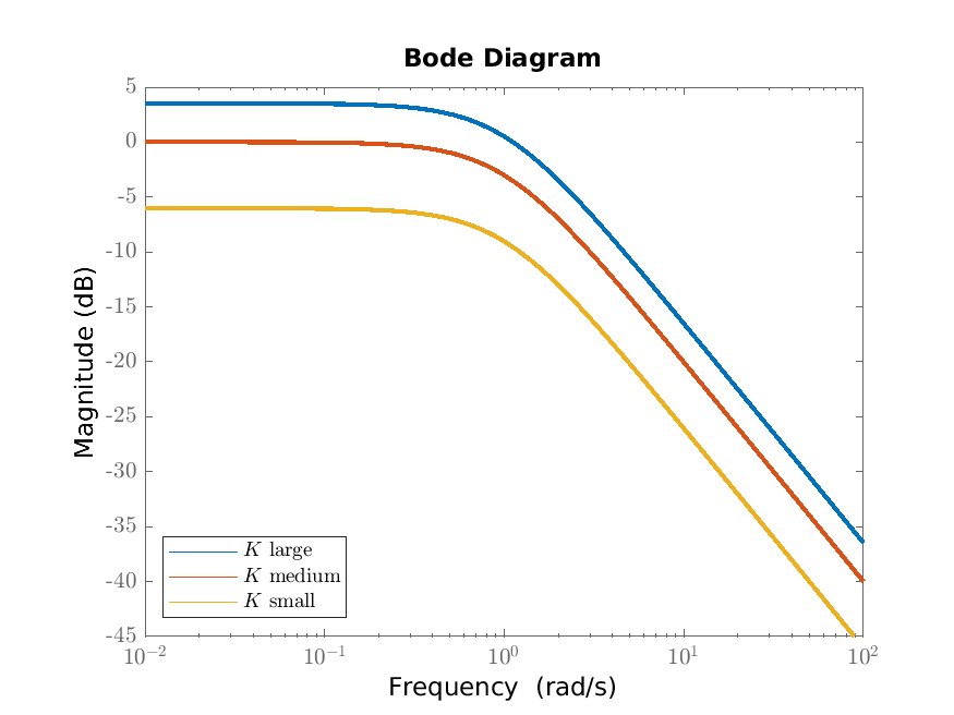
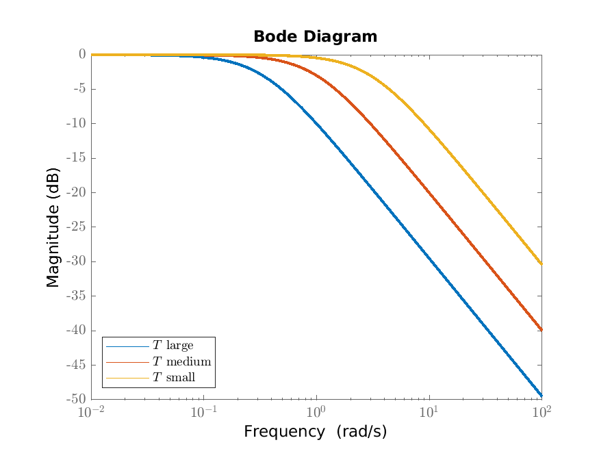
We consider plots of the frequency response of the first order scalar differential equation \(T\dot {y}(t)+y(t)=Ku(t)\) from Example 6.3. We plot this frequency response in Figures 6.1a (the Nyquist diagram) and 6.1b (the Bode diagram); the shape does not depend on the parameters \(K\) and \(T\) (through scaling). In Figures 6.2a and 6.2b we illustrate how the Bode magnitude diagram depend on the steady state gain \(K\) and the time constant \(T\).
We consider plots of the frequency response of the second order scalar differential equation
\[ T^2\ddot {q}(t)+2\zeta T\dot {q}(t)+q(t)=Ku(t),\quad y=q, \]
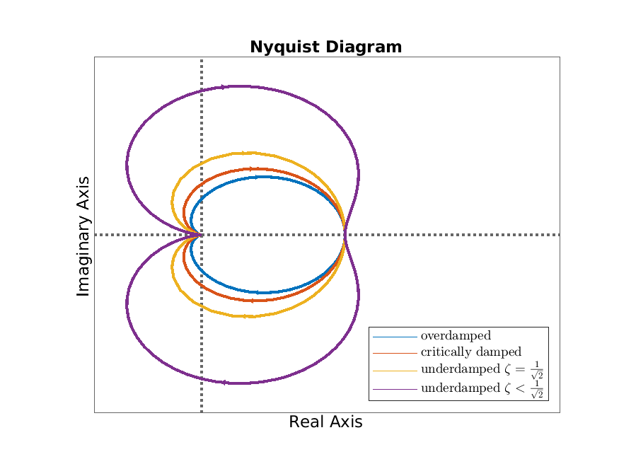
from Example 6.4. The Nyquist diagrams for relevant values of \(\zeta \) are given in Figure 6.3a. The bode diagrams for relevant values of \(\zeta \) are given in Figure 6.3b.
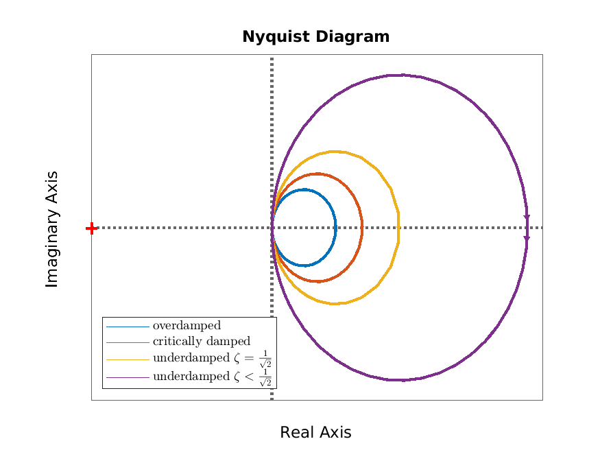
We consider plots of the frequency response of the second order scalar differential equation
\[ T^2\ddot {q}(t)+2\zeta T\dot {q}(t)+q(t)=Ku(t),\qquad y(t)=\dot {q}(t), \]
The Nyquist diagram is in Figure 6.4a and the Bode diagram in Figure 6.4b.
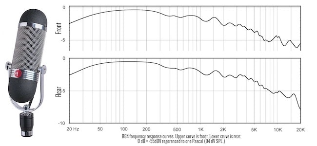
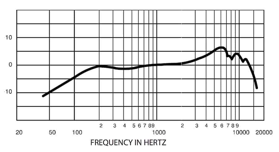
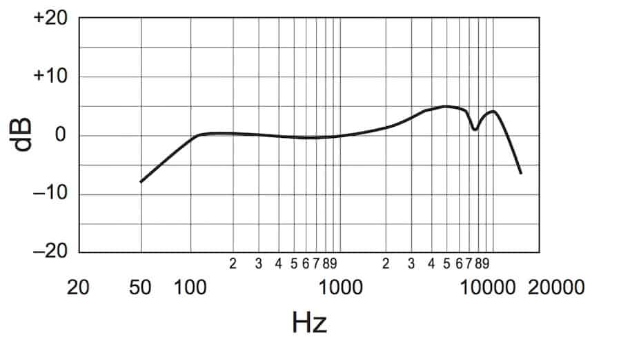
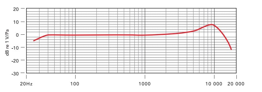
6.3 Case study: microphones*
A microphone operates as follows. Sound is a pressure wave in air. This causes a diaphragm (which is essentially a mass-spring-damper system) to vibrate. This vibration is then converted into an electrical signal. This is done either through an inductor based conversion (this is done in what are called dynamic microphones) or through a capacitor based conversion (this is done in what are called condenser microphones). Behind the diaphragm there is a small cavity (called the air gap) which is connected by tubes to a larger cavity (called the back cavity).
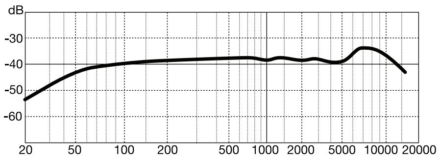
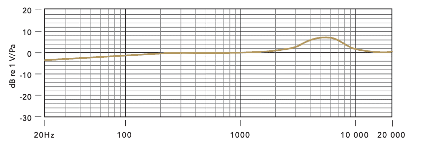
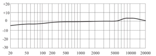
In Figure 6.5 we give the Bode magnitude diagrams of several microphones as provided by their manufacturers. The hearing range of humans is 20 Hz to 20,000 Hz (which is why this is the range on the horizontal axis). Typically for a microphone we want the Bode magnitude diagram to be approximately constant over this frequency range: this means that all frequencies are equally represented in the recording made through the microphone as they are in the live performance.
6.4 Case study: control of a tape drive*
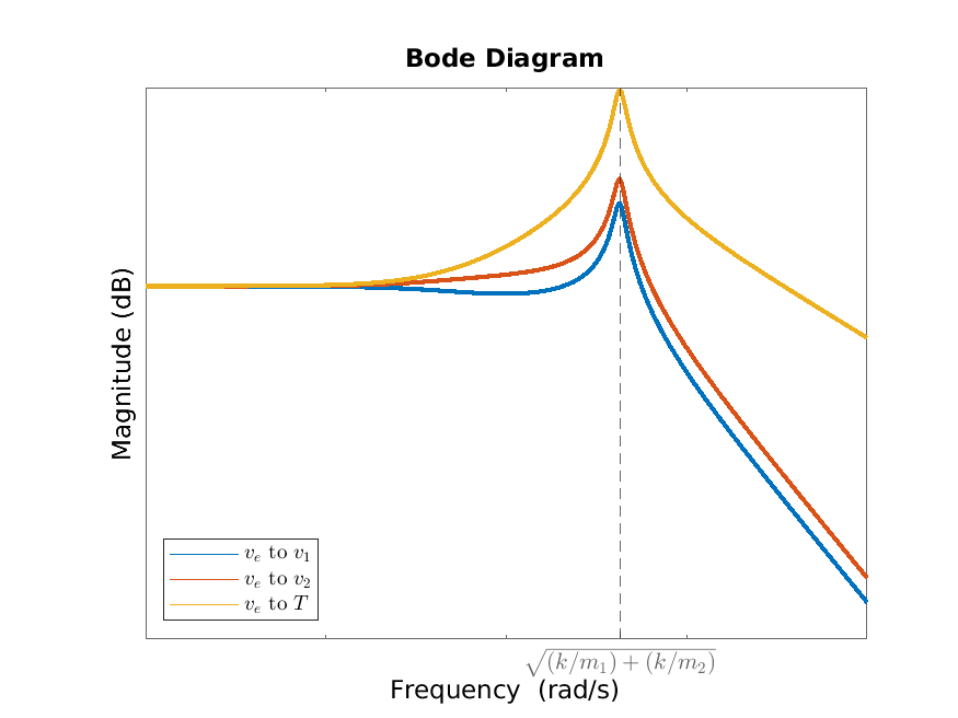
In Figure 6.6 we plot the frequency response from the disturbance \(v_e\) to each of the state variables \(v_1\), \(v_2\) and \(T\). Note that we already calculated the corresponding transfer functions in Section 5.2. We also indicated the approximate location of the peak of each of the frequency responses, namely
\(\seteqnumber{0}{6.}{0}\)\begin{equation} \label {eq:tapedrivefreq} \sqrt {\frac {k}{M_1}+\frac {k}{M_2}}, \end{equation}
which is the natural frequency of an undamped mass-spring system with spring constant \(k\) and mass
\[ \frac {1}{\frac {1}{M_1}+\frac {1}{M_2}}, \]
(you might recognize this way of “adding” the masses as the same as adding parallel resistances).
From the Bode magnitude diagram we can see at which frequencies a periodic disturbance of the form \(v_e(t)=\sin (\omega t)\) is most detrimental, namely for frequencies around the peak, so close to the frequency (6.1).
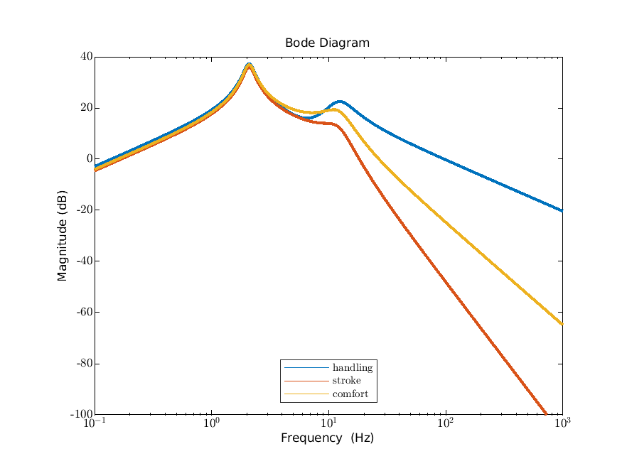
6.5 Case study: a suspension system*
We consider the fixed structure suspension system. In Figure 6.7 we give the Bode magnitude diagram from the road velocity to each of the three performance outputs. Here we have chosen values for the various physical parameters as in the introduction. On the horizontal axis the frequency is given in terms of Hertz rather than radians per second. An input of \(\sin (\omega t)\) corresponds to a sinusoidal road velocity, and therefore a sinusoidal road profile, namely \(\frac {-1}{\omega }\cos (\omega t)\) as a function of time \(t\). Noting that \(t=x/V\) where \(V\) is the horizontal velocity of the car (i.e. the speed we are travelling at), the corresponding road profile as a function of position \(x\) is \(\frac {-1}{\omega }\cos \left (\frac {\omega }{V}x\right )\). This can be thought of as representing an infinite sequence of equally spaced speedbumps. If we write \(\omega _0=\frac {\omega }{V}\), then the road profile is \(\frac {-1}{\omega _0V}\cos (\omega _0 x)\) and therefore \(\omega _0\) is related to the distancing of the speed bumps and \(\omega =\omega _0 V\) depends on both this spacing and on the speed of the car. So to find the relevant value of \(\omega \) in Figure 6.7 we have to consider both the distancing of the speed bumps and the speed of the car.
In Figure 6.7 we see that the Bode diagram has two “peaks” which correspond roughly to complex conjugate pairs of eigenvalues of the matrix \(A\) in the input-state-output system (or equivalently: poles of the transfer function). There is a clear peak around 2 Hz which in the automotive industry is called vehicle heave. This is because it is essentially due to the sprung mass and spring: we note that \(\frac {1}{2\pi }\sqrt {\frac {k_s}{m_s}}\approx 2.5\) Hz, which is the natural frequency of the subsystem consisting of only the sprung mass and spring. There is also a notable peak around 10 Hz which in the automotive industry is called wheel hop (or tyre hop). We note that \(\frac {1}{2\pi }\sqrt {\frac {k_{us}+k_s}{m_{us}}}\approx 12\) Hz, which is the natural frequency of the subsystem consisting of only the unsprung mass and both springs.
Assume a given spacing of speedbumps and consider what happens if we increase the speed \(V\) of the car (so that \(\omega =\omega _0 V\) increases). As we increase the speed up to where vehicle heave occurs, the amplification factor \(|F(\omega )|\) increases. This will make driving over these speedbumps less comfortable. Once we pass the point where vehicle heave occurs, the amplification factor \(|F(\omega )|\) decreases again. However, for handling, it starts to increase again around the frequency where wheel hop occurs (and after that it decreases again).
From the transfer functions computed in Section 5.3, we see that all three frequency responses are zero in zero, which we indeed see in Figure 6.7. The handling transfer function behaves like \(s^{-1}\) near infinity, the suspension stroke transfer function like \(s^{-3}\) and the comfort transfer function like \(s^{-2}\). In Figure 6.7 (since we have a loglog scale), we can see these powers \(-1\), \(-3\) and \(-2\) respectively in the slope for large frequencies.