Chapter 4 The step response
Recall that the step response \(H:[0,\infty )\phantom {]}\to \mR ^{p\times m}\) of \(\dot {x}=Ax+Bu\), \(y=Cx+Du\) is defined by
\[ \int _0^t C\e ^{A\theta }B\,d\theta +D. \]
Recall the variation of parameters formula (where in comparison to (2.2) we have made the substitution \(\theta \leftrightarrow t-\theta \) in the integral)
\(\seteqnumber{0}{4.}{0}\)\begin{equation} \label {eq:varpary2} y(t)=C\e ^{At}x^0+\int _0^t C\e ^{A\theta }Bu(t-\theta )\,d\theta +Du(t). \end{equation}
In the case that \(m=1\) (i.e. \(u\) is scalar-valued), we see from this that when \(x^0=0\) and \(u=1\) we obtain \(y=H\). This is where the name step response comes from: it is the response (i.e. the output) when the input is a unit step function (the convention is that functions are extended to the whole of \(\mR \) by definining them to be zero for negative time, so \(u(t)=0\) for \(t<0\) and \(u(t)=1\) for \(t>0\) which is indeed the unit step function).
If \(m>1\) (i.e. \(u\) is genuinely vector-valued), the the above applies column-wise. For example if \(m=2\), then we take \(x^0=0\), \(u_1=1\) and \(u_2=0\) to obtain the first column of the step response and we take \(x^0=0\), \(u_1=0\) and \(u_2=1\) to obtain the second column of the step response.
-
Remark 4.1. The above method of solving the differential equation with \(x^0=0\) and \(u=1\) is usually the best way of calculating the step response since it avoids forming the matrix exponential function. In the case of a higher order differential equation, using this method, it is not even needed to form the matrices \(A\), \(B\), \(C\) and \(D\) in order to calculate the step response.
4.1 Examples
-
Example 4.2. The step response of the first order scalar differential equation
\[ \dot {x}+x=u, \]
can be calculated by solving this equation with \(x(0)=0\) and \(u=1\), i.e. by solving
\[ \dot {x}+x=1,\qquad x(0)=0. \]
The homogeneous equation \(\dot {x}+x=0\) has general solution \(a\e ^{-t}\) and a particular solution of \(\dot {x}+x=1\) is \(x=1\). Therefore the general solution of \(\dot {x}+x=1\) is \(x(t)=1+a\e ^{-t}\). From the initial condition we obtain \(a=-1\) so that \(x(t)=1-\e ^{-t}\). Therefore \(H(t)=1-\e ^{-t}\) is the step response.
-
Example 4.3. We calculate the step response of the second order scalar differential equation
\[ \ddot {q}+\dot {q}+q=u,\qquad y=q. \]
We solve
\[ \ddot {q}+\dot {q}+q=1,\qquad q(0)=0,\quad \dot {q}(0)=0. \]
A particular solution is \(q=1\). The homogeneous equation is
\[ \ddot {q}+\dot {q}+q=0. \]
The characteristic polqnomial of this is \(s^2+s+1\), which has roots \(\frac {-1\pm i\sqrt {3}}{2}\), so that the general solution of the homogeneous equation is
\[ \e ^{-t/2}\left (a \cos \left (\frac {\sqrt {3}}{2}t\right )+b \sin \left (\frac {\sqrt {3}}{2}t\right )\right ). \]
adding the particular solution gives the general solution of our original equation:
\[ q(t)=1+\e ^{-t/2}\left (a \cos \left (\frac {\sqrt {3}}{2}t\right )+b \sin \left (\frac {\sqrt {3}}{2}t\right )\right ). \]
We now use the (zero) initial conditions to determine the constants \(a\) and \(b\). We have
\[ 0=q(0)=1+a,\quad 0=\dot {q}(0)=\frac {-1}{2}a+\frac {\sqrt {3}}{2}b. \]
This gives \(a=-1\) and \(b=\frac {-1}{\sqrt {3}}\). Therefore the step response is
\[ H(t)=1+\e ^{-t/2}\left (-\cos \left (\frac {\sqrt {3}}{2}t\right )-\frac {1}{\sqrt {3}} \sin \left (\frac {\sqrt {3}}{2}t\right )\right ). \]
-
\[ \dot {y}_1=y_2-u_2,\qquad \dot {y}_2+y_1=u_1. \]
Since \(m=p=2\), the step response has values in \(\mR ^{2\times 2}\). We determine the step response column-by-column. We first consider \(u_1=1\) and \(u_2=0\) (and zero initial condition). This gives
\[ \dot {y}_1=y_2,\qquad \dot {y}_2+y_1=1,\qquad y_1(0)=0,\quad y_2(0)=0. \]
We can rewrite this as the second order equation (we could alternatively solve the system of equations using matrix methods):
\[ \ddot {y}_1+y_1=1,\qquad y_1(0)=0,\quad \dot {y}_1(0)=0. \]
a particular solution is \(y_1=1\). The homogeneous equation is \(\ddot {y}_1+y_1=0\) and has general solution \(a\cos (t)+b\sin (t)\). Therefore the general solution of our original equation is
\[ 1+a\cos (t)+b\sin (t). \]
From the zero initial conditions we obtain \(1+a=0\), \(b=0\). Therefore we obtain
\[ y_1(t)=1-\cos (t). \]
We then calculate \(y_2=\dot {y}_1=\sin (t)\). Therefore the first column of the step response matrix is
\[ \bbm {1-\cos (t)\\\sin (t)}. \]
To obtain the second column of the step response matrix, we consider \(u_1=0\) and \(u_2=1\) (and zero initial conditions). This gives
\[ \dot {y}_1=y_2-1,\qquad \dot {y}_2=-y_1,\qquad y_1(0)=0,\quad y_2(0)=0. \]
a particular solution is \(y_2=1\), \(y_1=0\). The homogeneous equation is
\[ \dot {y}_1=y_2,\qquad \dot {y}_2=-y_1, \]
which we can write as the second order scalar differential equation
\[ \ddot {y}_1=-y_1, \]
the general solution of which is \(y_1(t)=a\cos (t)+b\sin (t)\). This gives \(y_2(t)=\dot {y}_1(t)=-a\sin (t)+b\cos (t)\). Therefore the general solution of the original equation is
\[ y_1(t)=a\cos (t)+b\sin (t),\qquad y_2(t)=1-a\sin (t)+b\cos (t). \]
We now determine \(a\) and \(b\) from the zero initial conditions. This gives \(a=0\), \(1+b=0\). Therefore
\[ y_1(t)=-\sin (t),\qquad y_2(t)=1-\cos (t). \]
It follows that the second column of the step response is
\[ \bbm {-\sin (t)\\1-\cos (t)}. \]
Hence the step response is
\[ H(t)=\bbm {1-\cos (t)&-\sin (t)\\\sin (t)&1-\cos (t)}. \]
We can alternatively use the formula from Definition 2.3. We write our system of equations in matrix form, with \(x:=y\), as
\[ \dot {x}=\bbm {0&1\\-1&0}x+\bbm {0&-1\\1&0}u,\qquad y=x. \]
Therefore
\[ A=\bbm {0&1\\-1&0},\qquad B=\bbm {0&-1\\1&0},\qquad C=\bbm {1&0\\0&1},\qquad D=\bbm {0&0\\0&0}. \]
The matrix exponential function of \(A\) is (the second year module MA20220 Ordinary Differential Equations and Control gave several different ways of calculating this):
\[ \e ^{At}=\bbm {\cos (t)&\sin (t)\\-\sin (t)&\cos (t)}. \]
We therefore have
\(\seteqnumber{0}{4.}{1}\)\begin{align*} H(t)&=\int _0^t C\e ^{A\theta }B\,d\theta +D =\int _0^t\bbm {\cos (\theta )&\sin (\theta )\\-\sin (\theta )&\cos (\theta )}\bbm {0&-1\\1&0}\,d\theta =\int _0^t \bbm {\sin (\theta )&-\cos (\theta )\\\cos (\theta )&\sin (\theta )}\,d\theta \\&=\bbm {1-\cos (t)&-\sin (t)\\\sin (t)&1-\cos (t)}, \end{align*} which is the same as we computed above in a column-by-column fashion.
4.2 Figures*
-
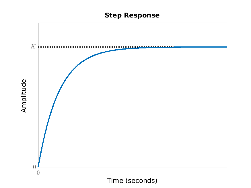
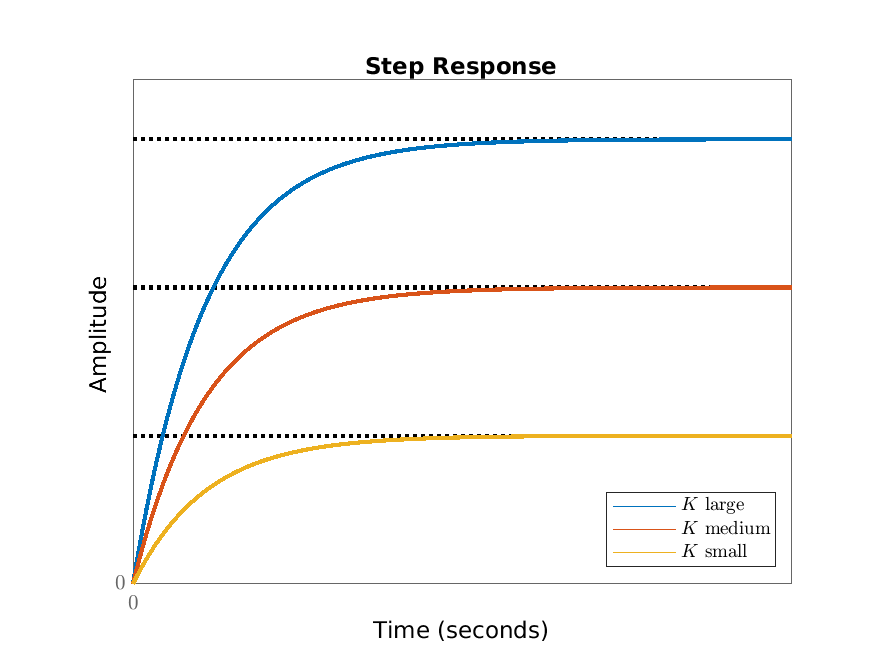
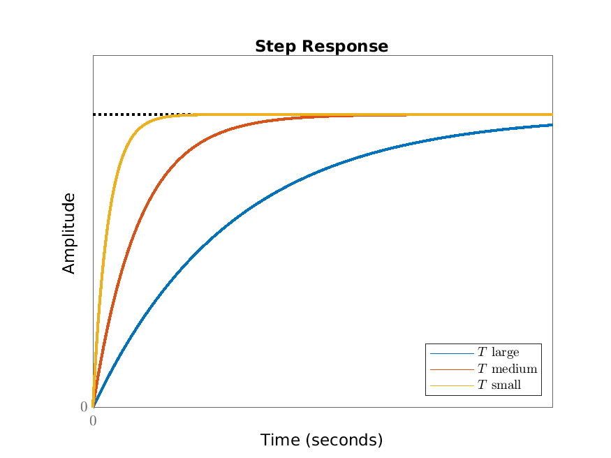
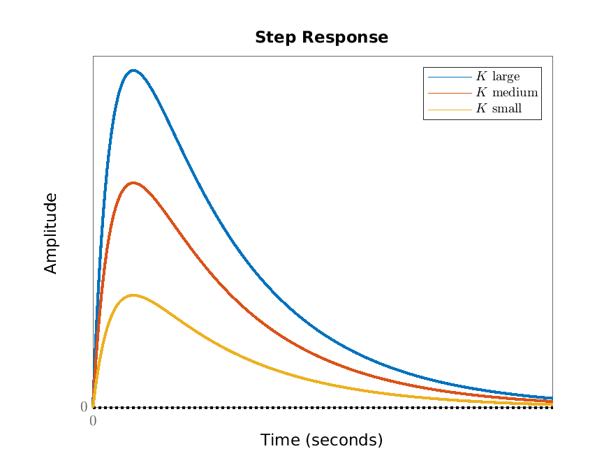
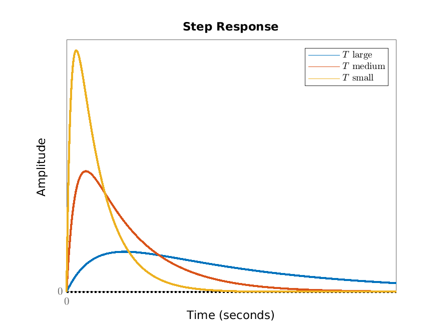
Example 4.5. Undoing the re-scaling in Example 4.2, we have that the step response of \(T\dot {x}+x=Ku\) (where \(T,K>0\)) is \(H(t)=K(1-\e ^{-t/T})\). The basic shape of this step response does not depend on \(K\) and \(T\) (since they scale out) and is given in Figure 4.1. The parameter-dependence is illustrated in Figure 4.2.
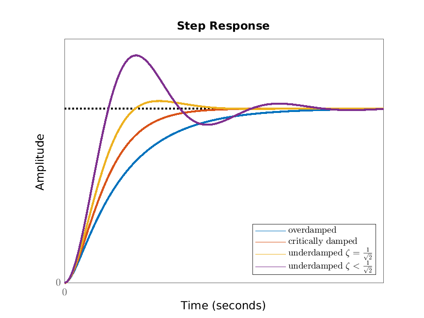
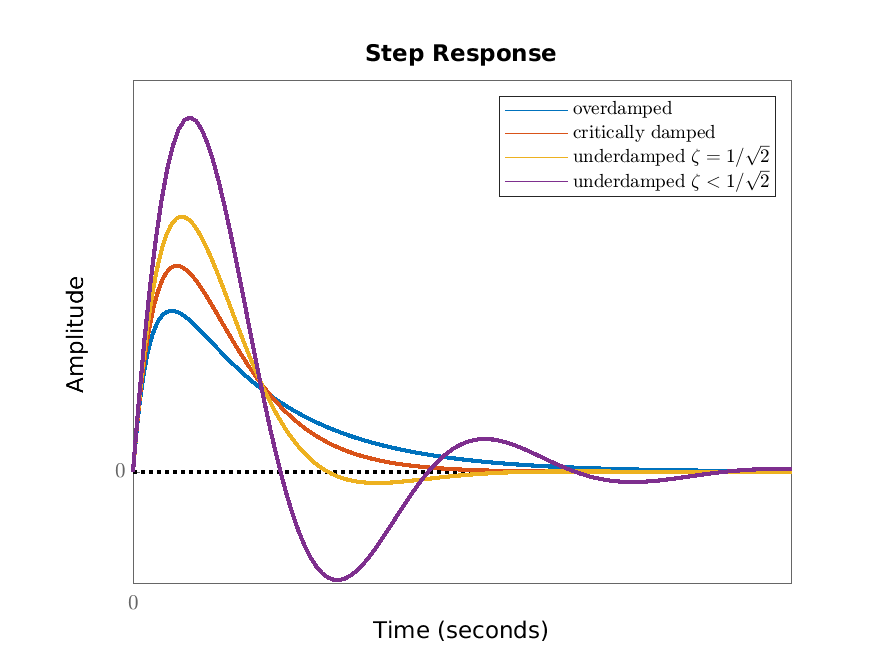
The step response of the second order scalar differential equation \(\ddot {q}+2\zeta \dot {q}+q=u\), \(y=q\) is given in Figure 4.3.
The step response of the second order scalar differential equation \(\ddot {q}+2\zeta \dot {q}+q=u\), \(y=\dot {q}\) is given in Figure 4.4.
In the overdamped case we consider the dependence of the step response of the second order scalar differential equation \(T^2\ddot {q}+2\zeta T\dot {q}+q=Ku\), \(y=\dot {q}\) on the parameters \(K\) and \(T\) in Figure 4.5.
4.3 Real-world examples*
-
Example 4.6. Consider a mass-spring-damper system with a force input and position output:
\[ m\ddot {y}+d\dot {y}+ky=u. \]
We can write this in the standard form \(T^2\ddot {q}+2\zeta T\dot {q}+q=Ku\), \(y=q\), where
\[ K=\frac {1}{k},\qquad T=\sqrt {\frac {m}{k}},\qquad \zeta =\frac {d}{2\sqrt {km}}. \]
Consider the situation where the mass is suspended from the (fixed) ceiling to which it is attached by the spring and damper. Assume that at time zero the system is supported from below to be at its equilibrium position. At time zero this support is removed and the constant gravitational force \(u=mg\) now acts on it. The output then is the step response multiplied by \(mg\). The new equilibrium position then is the steady state gain times this constant force: \(\frac {mg}{k}\) (we measure \(y\) as being positive towards the ground). If the damping constant is large, so that \(\zeta >1\) (the overdamped case), then convergence to this new equilibrium value is monotonic. If the damping constant is small (so that \(\zeta \in (0,1)\)), then the mass overshoots the new equilibrium on its approach.
4.4 Case study: diagnosis of lung diseases*
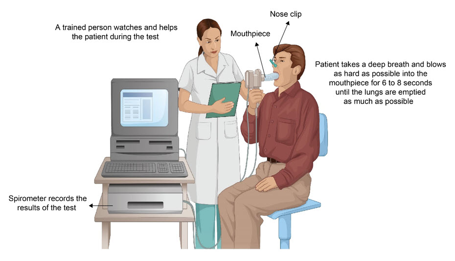
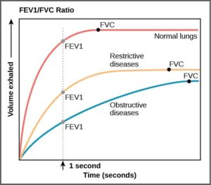
One method of diagnosing lung diseases (and distinguishing between two common types of lung diseases) is spirometry (see Figure 4.6a). There a patient blows as hard as possible for 6 to 8 second and the volume exhaled is measured. That the patient blows as hard as possible is not actually so crucial, more important is that the blowing is at a constant level (and the easiest way to make sure of this is to ask the patient to blow as hard as possible). The blowing acts as an input and the volume exhaled is the output. Since the blowing is at a constant level, the input is a step (or at least: the first 6 to 8 seconds of a step) and therefore the output is the step response (or at least: the first 6 to 8 seconds of the step response). The underlying input-state-output system is the lungs. Therefore what spirometry measures is the step response of the lungs of the patient. Note that the step response uniquely characterizes the input-output behavior, so even though spirometry seems restricted to one very specific input (blowing as hard as possible for 6 to 8 seconds), it actually captures the entire input-output behavior of the lungs.
From Figure 4.6b we see that the lungs are essentially a first order system (comparing the shapes of the graphs to Figure 4.1). Comparing Figure 4.6b to Figure 4.2a we see that for restrictive lung diseases the steady state gain is lower than normal (whereas the time constant is the same as normal). In Figure 4.6b we also see that for obstructive lung diseases (such as asthma) the steady state gain is lower than normal; however the literature is not unanimous about this. Comparing Figure 4.6b to Figure 4.2b we see that for obstructive lung diseases (such as asthma) the time constant is larger than normal. This is consistent in the literature. So the combination of gain and time constant distinguishes normal lungs and two types of lung diseases.
In Figure 4.6b FVC stands for forced vital capacity and is what in general is called the steady state gain. FEV1 stands for forced expiratory volume in one second. The ratio FEV1/FVC is equivalent to the time constant (in the sense that one can be uniquely computed from the other). What is more commonly measured is the ratio FEV1/FEV6 which is also equivalent to the time constant (the important thing is that we look at a ratio so that the steady state gain cancels).
4.5 Case study: muscle energy*
To perform work, the muscles need energy. This can be provided through the aerobic energy system (which needs oxygen) and through two anaerobic energy systems (which do not need oxygen). To investigate these energy systems, experimenters put someone on a stationary bike and ask them to put in a maximal effort for about 100 seconds. The cyclist is attached to various devices for measurement purposes. That the effort is maximal is not crucial, important is that the effort is constant (and an easy way to achieve this is to ask for maximal effort). The input then is a step and therefore the measurements give the step response of the three energy systems. These are given in Figure 4.7a.
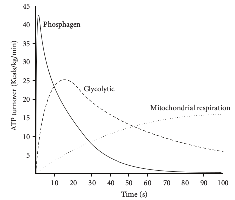
The aerobic energy system (labelled “mitochindrial respiration” in Figure 4.7a) is a first order system (as we essentially already saw in a different context in Section 4.4). The two anaerobic energy systems (labelled “phosphagen” and “glycolytic” in Figure 4.7a) have step responses of overdamped second order scalar differential equations of the form \(T^2\ddot {q}+2T\zeta \dot {q}+q=Ku\), \(y=\dot {q}\). Comparing to Figure 4.5b, we see that the phosphagen (or alactic) energy system has a smaller time constant than the glycolytic (or lactic) energy system.
That the glycolytic (or lactic) energy system is an overdamped second order scalar differential equations of the form \(T^2\ddot {q}+2T\zeta \dot {q}+q=Ku\), \(y=\dot {q}\) can be explained as follows. Denote the power produced by the lactic system by \(P\). The differential equation for \(P\) then is
\[ T_1\dot {P}+P+L=K_1u. \]
This is a standard first order scalar differential equation with time constant \(T_1\) and gain \(K_1\), except for the presence of term \(L\). This term represents the lactic acid in the muscles which inhibits power production by the lactic energy system. Lactic acid accumulates due to earlier power produced:
\[ T_2\dot {L}=P. \]
Differentiating the equation for \(L\) and substituting the equation for \(P\) gives
\[ T_1T_2\ddot {L}+T_2\dot {L}+L=K_1u,\qquad P=T_2\dot {L}. \]
Defining \(q:=T_2L\), this is a second order scalar differential equation of the form \(T^2\ddot {q}+2T\zeta \dot {q}+q=Ku\), \(y=\dot {q}\) with
\[ K=T_2K_1,\qquad T=\sqrt {T_1T_2},\qquad \zeta =\sqrt {\frac {T_2}{4T_1}}. \]
This is an overdamped system if and only if \(T_2>4T_1\).
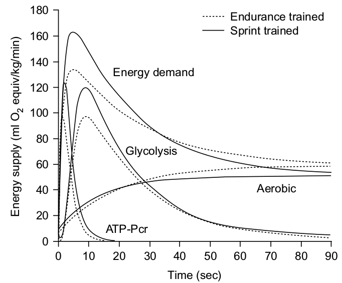
Figure 4.7b gives a comparison between sprinters and endurance athletes. We see that for the anaerobic systems the time constants seem similar, but the gain for the sprinters is higher. For the aerobic system (which is first order) the time constant for sprinters is smaller, but the steady state gain is lower. For the overall energy (labelled “energy demand” in Figure 4.7b) this results in sprinters being able to generate more power for the first 30 seconds, but less power after that.
In reality, lactic acid is probably removed during non-maximal exercise. This will make the system nonlinear.