Chapter 5 Inference for relationships
So far we have always considered one random sample \(X_1,\ldots,X_n\) from some density \(f(x|\theta)\). Very often we are interested in the differences in distributions between two or more random samples.
We first turn to the case where two random samples of continuous data are available.
Example 5.1 (ACTG175 trial, two sample comparison) Recall from Example 1.9 that the AIDS Clinical Trials Group Study 175 (ACTG175) was a randomised clinical trial conducted in the 1990s to compare different treatments for adults infected with HIV. The trial had four randomised groups, with each group receiving a different treatment. We will focus on a comparison of those randomised to receive zidovudine (532 patients) and those randomised to receive a combination treatment of zidovudine plus didanosine (522 patients). One of the outcomes is the patient’s CD4 blood cell count. A larger CD4 value is indicative that the treatment is working. Thus one of the analyses of interest is to compare the CD4 count after treatment with zidovudine plus didanosine compared to treatment with zidovudine alone. Figure 5.1 shows overlaid density plots of the CD4 count 20 weeks after baseline in these two groups.
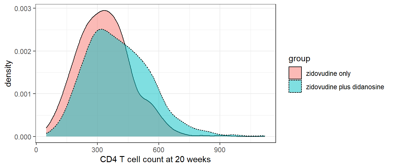
Figure 5.1: Distribution of CD4 T cell count at 20 weeks in zidovudine only versus zidovudine plus didanosine groups of ACTG175 trial
Visually there is some suggestion that the CD4 distribution is shifted towards larger values in the zidovudine plus didanosine group.
The comparison of these two treatment groups can be represented as a two-sample problem. In particular, our model will assume that the CD4 data on the patients in these two groups represent independent samples from the two hypothetical populations that would exist were we to treat all the eligible patients in the population with these two treatment options.
Example 5.2 (ACTG175 trial, paired sample) Sometimes the two groups might be composed of exactly the same individuals, the only difference being that they are observed at two different time-points. For example, in the ACTG175 trial, we may be interested in comparing the CD4 count at baseline (before treatment) to the week 20 CD4 count (after treatment), within one of the randomised groups. Figure 5.2 shows the histogram of change in CD4 from baseline to 20 weeks (20 week value minus baseline value) in the zidovudine plus didanosine group.
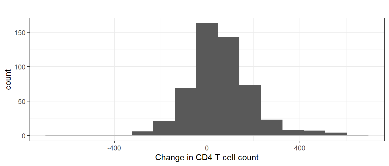
Figure 5.2: Histogram of change in CD4 T cell count from baseline to 20 weeks in zidovudine plus didanosine group of ACTG175 trial
The first example above corresponds to a situation where we normally assume that the random samples corresponding to two different groups of individuals can be considered to be independent. In the second example, the observations are clearly paired (and therefore dependent) since we can arrange the observations as pairs (before and after) corresponding to each individual. In fact, it would be more accurate to describe the second example as a one-sample bivariate setting, rather than a two-sample setting. We treat the cases of inference for independent and dependent (paired) samples separately.
5.1 Independent samples - comparing means
We now consider comparisons of the means \(\mu_{X}\) and \(\mu_{Y}\) in the two groups. Suppose we assume again that the distributions are normal, with \(X_{1}, \ldots, X_{n}\) i.i.d. from \(N(\mu_{X},\sigma_{X}^{2})\), and \(Y_{1}, \ldots, Y_{m}\) i.i.d. from \(N(\mu_{Y}, \sigma^{2}_{Y})\). Note that in general \(n\) need not equal \(m\).
5.1.1 Variances known
Consider first the unrealistic case that both \(\sigma^{2}_{X}\) and \(\sigma^{2}_{Y}\) are known. We know that \(\overline{X} \sim N(\mu_{X}, \sigma^{2}_{X}/n)\) and \(\overline{Y} \sim N(\mu_{Y}, \sigma^{2}_{Y}/m)\). Then since the two groups are independent, it follows from the properties of linear combinations of normal random variables that \[\begin{equation} \overline{X}-\overline{Y} \sim N\left(\mu_{X} - \mu_{Y}, \frac{\sigma^{2}_{X}}{n} + \frac{\sigma^{2}_{Y}}{m}\right). \tag{5.1} \end{equation}\] This result can readily be used to form confidence intervals for and perform hypothesis tests concerning the difference in means \(\mu_{X}-\mu_{Y}\).
CONFIDENCE INTERVAL
To construct a \(100 \times (1-\alpha)\)% confidence interval for \(\mu_{X}-\mu_{Y}\), first we note that: \[\begin{eqnarray*} \frac{\overline{X}-\overline{Y} - (\mu_{X}-\mu_{Y})}{\sqrt{\frac{\sigma^{2}_{X}}{n} + \frac{\sigma^{2}_{Y}}{m}}} \sim N(0,1) \end{eqnarray*}\] is a pivot for \(\mu_{X}-\mu_{Y}\). Thus \[\begin{eqnarray*} P\left(-z_{1-\alpha/2} < \frac{\overline{X}-\overline{Y} - (\mu_{X}-\mu_{Y})}{\sqrt{\frac{\sigma^{2}_{X}}{n} + \frac{\sigma^{2}_{Y}}{m}}} < z_{1-\alpha/2} \right) = 1-\alpha \end{eqnarray*}\] Then re-arranging the inequality and multiplying through by \(-1,\) we have \[\begin{eqnarray*} P\left( \overline{X}-\overline{Y} - z_{1-\alpha/2} \sqrt{\frac{\sigma^{2}_{X}}{n} + \frac{\sigma^{2}_{Y}}{m}} < \mu_{X}-\mu_{Y} < \overline{X}-\overline{Y} + z_{1-\alpha/2} \sqrt{\frac{\sigma^{2}_{X}}{n} + \frac{\sigma^{2}_{Y}}{m}} \right) = 1-\alpha \end{eqnarray*}\] Given some observed data, a \(100 \times (1-\alpha)\)% confidence interval for \(\mu_{X}-\mu_{Y}\) is thus given by \[\begin{eqnarray*} \overline{x}-\overline{y} \pm z_{1-\alpha/2} \sqrt{\frac{\sigma^{2}_{X}}{n} + \frac{\sigma^{2}_{Y}}{m}}. \end{eqnarray*}\]
HYPOTHESIS TESTING
Now consider hypothesis tests concerning \(\mu_{X}-\mu_{Y}\). A natural null hypothesis is that \(\mu_{X}-\mu_{Y}=0\), or equivalently that \(\mu_{X}=\mu_{Y}\). Under this null: \[\begin{eqnarray*} Z = \frac{\overline{X}-\overline{Y}}{\sqrt{\frac{\sigma^{2}_{X}}{n} + \frac{\sigma^{2}_{Y}}{m}}} \sim N(0,1) \end{eqnarray*}\] Following the one-sample setting, we can construct significance level \(\alpha\) tests for one-sided or two-sided alternatives are shown in Table 5.1
| \(H_0\) | vs. \(H_1\) | Reject \(H_0\) if |
|---|---|---|
| \(\mu_X=\mu_Y\) | \(\mu_X>\mu_Y\) | \(z \geq z_{1-\alpha}\) |
| \(\mu_X=\mu_Y\) | \(\mu_X<\mu_Y\) | \(z \leq -z_{1-\alpha}=z_{\alpha}\) |
| \(\mu_X=\mu_Y\) | \(\mu_X\neq\mu_Y\) | \(|z| \geq z_{1-\alpha/2}\) |
5.1.2 Variances unknown, assumed equal
More typically, the two variances \(\sigma^{2}_{X}\) and \(\sigma^{2}_{Y}\) will be unknown. There are two routes for proceeding, based on whether we assume the two variances are equal. One could test the null hypothesis of equality of variances using the theory described later in Section 5.3 and proceed according to whether this test indicates evidence of inequality. However, this is generally inadvisable. For one thing, the power of this test may be low, such that we may accept the null of equal variances with high probability even when the variances differ.
One generally accepted rule of thumb is to assume equal variances if the ratio of the larger sample variance to the smaller is no more than two. But even in this case, some statisticians defer to methods that to allow them to be different. Having said all this, let us now proceed to examine comparison of the means under the assumption that \(\sigma^{2}_{X}=\sigma^{2}_{Y}=\sigma^{2}\), again under the assumption that the true distribution in each group is normal.
We first have to estimate the common variance \(\sigma^{2}\) using the data. We know that the usual \(S^{2}\) estimator applied to each group is unbiased for \(\sigma^{2}\). We therefore pool the \(S^{2}\) estimates from the two groups to form a combined estimate of \(\sigma^{2}\). We estimate \(\sigma^{2}\) from each group’s data and average them, weighting according to their respective sample sizes.
Definition 5.1 (Pooled variance estimator) The pooled estimator of the common variance \(\sigma^2\) is defined as: \[\begin{equation} S_{p}^{2} = \frac{(n-1)S_{X}^{2} + (m-1)S_{Y}^{2}}{n+m-2}. \tag{5.2} \end{equation}\]
Note that we cannot simply calculate \(S^{2}\) in the combined sample, \(\{X_1, \dots X_n, Y_1, \dots Y_m\}\), since this estimates the variability of the sample around the pooled sample mean, a different quantity.
Next we establish the sampling distribution of \(S_{p}^{2}\) and of \(\overline{X}-\overline{Y}\).
Proposition 5.1 Let \(X_{1},\dots,X_{n}\) be i.i.d. \(N(\mu_{X},\sigma^{2})\) and \(Y_{1},\dots,Y_{m}\) be i.i.d. \(N(\mu_{Y},\sigma^{2})\), with the two samples independent. Then \[\begin{eqnarray*} \frac{n+m-2}{\sigma^{2}} S^{2}_{p} \sim \chi^{2}_{n+m-2} \end{eqnarray*}\] and \[\begin{eqnarray*} \frac{\overline{X} - \overline{Y} - (\mu_{X}-\mu_{Y})}{S_{p}\sqrt{\displaystyle \frac{1}{n} + \frac{1}{m}}} \sim t_{n+m-2}. \end{eqnarray*}\]
Proof: From Theorem 3.1, we have that \[\begin{eqnarray*} \frac{n-1}{\sigma^{2}}S_{X}^{2} \sim \chi^{2}_{n-1}\qquad \mbox{and}\qquad\frac{m-1}{\sigma^{2}}S_{Y}^{2} \sim \chi^{2}_{m-1} \end{eqnarray*}\] As \(S_{X}^{2}\) and \(S_{Y}^{2}\) are independent, the sum \[\begin{eqnarray*} \frac{n-1}{\sigma^{2}} S_{X}^{2} + \frac{m-1}{\sigma^{2}} S_{Y}^{2} = \frac{n+m-2}{\sigma^{2}} S_{p}^{2} \end{eqnarray*}\] is the sum of two independent \(\chi^{2}\) random variables. Recalling from Probability & Statistics 1B that the \(\chi^{2}\) distribution is a special case of the gamma distribution (\(\chi^2_{\nu} = Ga(1/2, \nu/2)\)) and that the sum of two independent gamma random variables with shared scale parameter is also gamma, we have \[\begin{eqnarray*} \frac{(n+m-2) S_{p}^{2}}{\sigma^{2}} & \sim & \chi^{2}_{n+m-2}. \end{eqnarray*}\] Since the two samples are independent, we have that \[\begin{eqnarray*} \overline{X} - \overline{Y} \sim N\left(\mu_{X} - \mu_{Y}, \sigma^{2}\left(\frac{1}{n} + \frac{1}{m}\right)\right), \end{eqnarray*}\] and so \[\begin{eqnarray*} \frac{\overline{X} - \overline{Y} - (\mu_{X}-\mu_{Y})}{\sigma \sqrt{\frac{1}{n} + \frac{1}{m}}} \sim N\left(0, 1\right). \end{eqnarray*}\] Lastly, from Theorem 3.1, we have that \(S^{2}_{X}\) is independent of \(\overline{X}\), and similarly that \(S^{2}_{Y}\) is independent of \(\overline{Y}\). From this it follows that \(\overline{X}-\overline{Y}\) and \(S_p^2\) are independent, so from the definition of the t-distribution (Definition 3.4): \[\begin{eqnarray*} & & \frac{\overline{X} - \overline{Y} - (\mu_{X}-\mu_{Y})}{\sigma \sqrt{\frac{1}{n} + \frac{1}{m}}} \bigg/ (S_{p}/\sigma) \\ &=& \frac{\overline{X} - \overline{Y} - (\mu_{X}-\mu_{Y})}{S_{p}\sqrt{\displaystyle \frac{1}{n} + \frac{1}{m}}} \sim t_{n+m-2} \quad \square \end{eqnarray*}\]
This result can then be used to form confidence intervals for and test hypotheses concerning the difference in means \(\mu_{X}-\mu_{Y}\).
CONFIDENCE INTERVAL
Based on the conclusions of Proposition 5.1, analogously to the one sample situation considered in Section 3.2, we can form a \(100 \times (1-\alpha)\)% confidence interval for \(\mu_{X}-\mu_{Y}\) as \[\begin{eqnarray*} \overline{x}-\overline{y} \pm t_{n+m-2,1-\alpha/2} \times s_{p} \sqrt{\displaystyle \frac{1}{n} + \frac{1}{m}}. \end{eqnarray*}\]
HYPOTHESIS TESTING
Under \(H_{0}:\mu_{X}=\mu_{Y}\), we have from Proposition 5.1 that \[\begin{eqnarray*} T & = & \frac{\overline{X} - \overline{Y}}{S_{p}\sqrt{\displaystyle \frac{1}{n} + \frac{1}{m}}} \sim t_{n+m-2} \end{eqnarray*}\] We can use this to construct one-sided and two-sided tests with significance level \(\alpha\) as shown in Table 5.2.
| \(H_0\) | vs. \(H_1\) | Reject \(H_0\) if |
|---|---|---|
| \(\mu_X=\mu_Y\) | \(\mu_X>\mu_Y\) | \(t \geq t_{n+m-2,1-\alpha}\) |
| \(\mu_X=\mu_Y\) | \(\mu_X<\mu_Y\) | \(t \leq -t_{n+m-2,1-\alpha}\) |
| \(\mu_X=\mu_Y\) | \(\mu_X\neq\mu_Y\) | \(|t| \geq t_{n+m-2,1-\alpha/2}\) |
Example 5.3 We now consider comparing the mean CD4 count at week 20 in the ACTG175 study, assuming the two populations have a common unknown variance \(\sigma^{2}\).
We let the \(x_{1}, \ldots,x_{532}\) denote the observed CD4 counts in the zidovudine treatment group. The data is summarised by \[\begin{eqnarray*} n = 532; \ \sum_{i=1}^{532} x_{i} \ = \ 178826; \ \sum_{i=1}^{532} x_{i}^{2} = 69217556 \end{eqnarray*}\] so that \[\begin{eqnarray*} \overline{x} & = & \frac{1}{n} \sum_{i=1}^{n} x_{i} \ = \ \frac{178826}{532} \ = \ 336.14, \\ s_{x}^{2} & = & \frac{1}{n-1}\left(\sum_{i=1}^{n} x_{i}^{2} - n \overline{x}^{2} \right) \\ & = & \frac{1}{531}\left(69217556 - 532\left(\frac{178826}{532}\right)^{2}\right) \ = \ 17150.934. \end{eqnarray*}\] Similarly, let \(y_{1}, \ldots,y_{522}\) denote the values in the zidovudine plus didanosine group. The data is summarised by \[\begin{eqnarray*} m = 522; \ \sum_{i=1}^{522} y_{i} \ = \ 210456; \ \sum_{i=1}^{522} y_{i}^{2} = 97578584 \end{eqnarray*}\] so that \[\begin{eqnarray*} \overline{y} & = & \frac{1}{m} \sum_{i=1}^{m} y_{i} \ = \ \frac{210456}{522} \ = \ 403.17, \\ s_{y}^{2} & = & \frac{1}{m-1}\left(\sum_{i=1}^{m} y_{i}^{2} - m \overline{y}^{2} \right) \\ & = & \frac{1}{521}\left(97578584 - 522\left(\frac{210456}{522}\right)^{2}\right) \ = \ 24430.961. \end{eqnarray*}\] Our point estimate for the difference in mean CD4 count, \(\mu_{X}-\mu_{Y}\), is thus \(\overline{x}-\overline{y}=-67.03\). The pooled estimate of the common variance is \[\begin{eqnarray*} s_{p}^{2} & = & \frac{(n-1)s^{2}_{x} + (m-1)s^{2}_{y}}{n+m-2} \\ & = &\frac{(532-1)(17150.934)+(522-1)(24430.961)}{532+522-2} \ = \ 20756.346. \end{eqnarray*}\] A 95% confidence interval for \(\mu_{X}-\mu_{Y}\) is then \[\begin{eqnarray*} \overline{x}-\overline{y} \pm t_{1052,1-\alpha/2} \times s_{p} \sqrt{\displaystyle \frac{1}{532} + \frac{1}{522}} \end{eqnarray*}\] where \(t_{1052,1-\alpha/2}=1.962\) (using
qt(0.975,1052)). This gives \((-84.45, -49.62)\).We now perform a test of the hypothesis \(H_{0}:\mu_{X}=\mu_{Y}\) versus the two-sided alternative, at the 5% level. Our test statistic is \[\begin{eqnarray*} \frac{\overline{x} - \overline{y}}{s_{p}\sqrt{\displaystyle \frac{1}{n} + \frac{1}{m}}} \sim t_{n+m-2}& = &\frac{-67.03}{144.071\sqrt{1/532+1/522}} = -7.552. \end{eqnarray*}\] The corresponding \(p\)-value is \[\begin{eqnarray*} 2 \times P(T_{1052}\geq|-7.552|) = 0 \end{eqnarray*}\]
Given Figure 5.1 we should be concerned about the normality assumption. However, given the size of \(n\) and \(m\) here, we can be reasonably satisfied that the coverage of the confidence interval is close to 95% and the test’s Type I error is close to the desired 5% level, if we believe the assumption of a common variance is correct. Given our earlier estimates of the variances in the two groups, we have reason to doubt this assumption.
5.1.3 Variances unknown, possibly unequal
We now consider the most realistic situation in practice: we allow for the possibility the variances in the two groups may well not be equal, and we do not know their true values. Recall from Equation (5.1) that \[\begin{eqnarray*} \overline{X}-\overline{Y} \sim N\left(\mu_{X} - \mu_{Y}, \frac{\sigma^{2}_{X}}{n} + \frac{\sigma^{2}_{Y}}{m}\right), \end{eqnarray*}\] but now we do not know the values of \(\sigma^{2}_{X}\) and \(\sigma^{2}_{Y}\). From Proposition 2.2 we have that \(S^{2}_{X}\) and \(S^{2}_{Y}\) are consistent estimators of \(\sigma^{2}_{X}\) and \(\sigma^{2}_{Y}\) respectively, and so we can estimate \(\frac{\sigma^{2}_{X}}{n} + \frac{\sigma^{2}_{Y}}{m}\) by \(\frac{S^{2}_{X}}{n} + \frac{S^{2}_{Y}}{m}.\)
We then consider the distribution of
\[\begin{eqnarray*}
\frac{(\overline{X}-\overline{Y}) - (\mu_{X} - \mu_{Y})}{\sqrt{\frac{S^{2}_{X}}{n} + \frac{S^{2}_{Y}}{m}}}
\end{eqnarray*}\]
Unfortunately this distribution is not a standard one. One popular approach approximates the distribution with a t-distribution with a certain degrees of freedom, leading to Welch’s test, which is available in R. For carrying out
calculations by hand, we shall instead consider the asymptotic distribution
of this test statistic, which as we shall see, is standard normal.
Proposition 5.2 Let \(X_{1},\dots,X_{n}\) be i.i.d. \(N(\mu_{X},\sigma^{2}_X)\) and \(Y_{1},\dots,Y_{m}\) be i.i.d. \(N(\mu_{Y},\sigma^{2}_Y)\), with the two samples independent. Then assume that as \(n \rightarrow \infty\) and \(m \rightarrow \infty\), \(\frac{m}{n+m} \rightarrow \rho\) for some \(0<\rho<1\). Then \[\begin{eqnarray*} \frac{\overline{X}_{n}-\overline{Y}_{m} - (\mu_{X} - \mu_{Y})}{\sqrt{\frac{S^{2}_{X}}{n} + \frac{S^{2}_{Y}}{m}}} & \xrightarrow{L} & N\left(0, 1 \right). \end{eqnarray*}\]
Proof: See the non-examinable proofs chapter, Chapter 6.
Example 5.4 Continuing with the ACTG175 data, we now calculate a 95% confidence interval for the difference in treatment group means, relaxing the assumption that they have a common population variance. Using Proposition 5.2 we have an asymptotically valid 95% confidence interval given by \[\begin{eqnarray*} \overline{x}-\overline{y} \pm 1.96 \sqrt{\frac{s^{2}_{X}}{n} + \frac{s^{2}_{Y}}{m}} &=& -67.033 \pm 1.96 \sqrt{\frac{17150.934}{532} + \frac{24430.961}{522}} \\ &=& (-84.46, -49.61) \end{eqnarray*}\] which compares with the confidence interval calculated assuming a common variance of $(-84.45, -49.62). They are similar despite the quite different sample variances in the two groups because the groups are of similar size, such that the two estimated standard errors for the difference in sample means are very similar.
5.1.4 Asymptotic confidence intervals and tests
We have developed confidence intervals and hypothesis tests for comparing the two group means based on normality assumptions for \(X\) and \(Y\). In fact these procedures are robust to non-normality provided \(\sigma^{2}_{X}\) and \(\sigma^{2}_{Y}\) are finite – so that we can apply the CLT – and that we have consistent estimators \(\widehat \sigma^{2}_{X}\) and \(\widehat \sigma^{2}_{Y}\) of these variances – so that we can apply Slutsky.
Then in the equal variance case we have \[\begin{equation} \frac{\overline{X}_{n} - \overline{Y}_{m} - (\mu_{X}-\mu_{Y})}{S_{p}\sqrt{\displaystyle \frac{1}{n} + \frac{1}{m}}} \xrightarrow{L} N(0,1) \tag{5.3} \end{equation}\] where \[\begin{eqnarray*} S_{p}^{2} = \frac{(n-1)\widehat \sigma_{X}^{2} + (m-1)\widehat \sigma_{Y}^{2}}{n+m-2}. \end{eqnarray*}\] and in the un-equal variance case we have \[\begin{equation} \frac{\overline{X}_{n}-\overline{Y}_{m} - (\mu_{X} - \mu_{Y})}{\sqrt{\frac{\widehat \sigma^{2}_{X}}{n} + \frac{\widehat \sigma^{2}_{Y}}{m}}} \xrightarrow{L} N\left(0, 1 \right) \tag{5.4} \end{equation}\]
More formal statements and proofs for the claims in (5.3) and (5.4) are given in Chapter 6. Note that we do not require \(\widehat \sigma^{2}_{X} = S^2_X\) or \(\widehat \sigma^{2}_{Y} = S^2_Y\), though often these estimators of the variance are used in practice. Review 2.2 to remind yourself when \(S^2\) is a consistent estimator of the variance.
We can now exploit these results to construct confidence intervals and tests for particular (non-normal) distributions that asymptotically will have the correct coverage and size. How good the approximation is will depend on the magnitudes of \(n\) and \(m\) as well as how close the true data generating distributions in the two groups are to normals.
Example 5.5 (Bernoulli model) Let \(X_{1},\ldots,X_{n}\) be i.i.d. Bernoulli with success probability \(p_{X}\) and \(Y_{1},\ldots,Y_{m}\) be i.i.d. Bernoulli with success probability \(p_{Y}\). Since \(E(X)=p_{X}\) and \(E(Y)=p_{Y}\), we can use our preceding results for comparing means to compare \(p_{X}\) with \(p_{Y}\). We have \(\text{Var}(X)=p_{X}(1-p_{X}) < \infty\) and similarly \(\text{Var}(Y)<\infty\). Previously we considered the MLE of \(\text{Var}(X)=p_{X}(1-p_{X})\) which is \(\widehat{p_{X}}(1-\widehat{p_{X}})\), where \(\widehat{p_{X}}=\overline{X}\). This is a consistent estimator by the Weak Law of Large Numbers and Continuous Mapping Theorem.
Thus we can use Equation (5.4) to construct confidence intervals for \(p_{X}-p_{Y}\) and perform hypothesis tests. We have \[\begin{eqnarray*} \frac{\widehat{p_{X}}-\widehat{p_{Y}} - \left(p_X - p_Y\right)}{\sqrt{\frac{\widehat{p_{X}}(1-\widehat{p_{X}})}{n} + \frac{\widehat{p_{Y}}(1-\widehat{p_{Y}})}{m}}} & \xrightarrow{L} & N\left(0, 1 \right) \end{eqnarray*}\]
A \(100 \times (1-\alpha)\)% confidence interval for \(p_{X}-p_{Y}\) is then \[\begin{eqnarray*} \widehat{p_{X}} - \widehat{p_{Y}} \pm z_{1-\alpha/2} \sqrt{\frac{\widehat{p_{X}}(1-\widehat{p_{X}})}{n} + \frac{\widehat{p_{Y}}(1-\widehat{p_{Y}})}{m}} \end{eqnarray*}\]
To conduct a hypothesis test of the null hypothesis that \(p_{X}=p_{Y}\), we can observe that under this hypothesis \[\begin{eqnarray*} \frac{\widehat{p_{X}}-\widehat{p_{Y}}}{\sqrt{\frac{\widehat{p_{X}}(1-\widehat{p_{X}})}{n} + \frac{\widehat{p_{Y}}(1-\widehat{p_{Y}})}{m}}} & \xrightarrow{L} & N\left(0, 1 \right) \end{eqnarray*}\] This can be used to construct tests against one-sided or two-sided alternatives in the usual way.
The ‘standard’ large sample (asymptotic) test for this situation is actually based on a slightly different test statistic. Specifically, under the null that \(p_{X}=p_{Y}=p\), the common variance \(p(1-p)\) can be estimated by \(\check{p}(1-\check{p})\), where \(\check{p}=(\sum X_{i} + \sum Y_{i})/(n+m)\). This leads to the test-statistic: \[\begin{equation} \frac{\widehat{p_{X}}-\widehat{p_{Y}}}{\sqrt{\check{p}(1- \check{p}) \left(\frac{1}{n} + \frac{1}{m} \right)}} \tag{5.5} \end{equation}\] which again is asymptotically \(N(0,1)\) under the null.
Example 5.6 Recall from Example 1.10 that the Physician’s Health Study was a medical study carried out in the 1980s to investigate the benefits and risks of aspirin for cardiovascular disease and cancer. The trial randomised 22,071 healthy doctors to receive either aspirin or placebo. They were then followed-up to see who experienced heart attacks during the following 5 years. The data are shown again in Table 5.3.
Table 5.3: Number of heart attacks by treatment group in the Physician's Health Study. Group Heart attack No heart attack Total Aspirin 139 10898 11037 Placebo 239 10795 11034 Primary interest is in whether receiving aspirin increased or decreased the probability of experiencing a heart attack. We can model this using the two-sample Bernoulli model considered in the preceding example. Thus we let \(X_{i}\) denote the heart attack outcome (1=yes, 0=no) for the \(i\)th participant in the aspirin group, and \(Y_{i}\) denote the heart attack outcome in the \(i\)th participant in the placebo group.
The estimated 5-year risk of a heart attack for the aspirin group is \(139/11037 = 0.013\). The estimated 5-year risk of a heart attack for the placebo group is \(239/11034 = 0.022\). The estimated difference in probability of heart attack (aspirin minus placebo) is thus \[\begin{eqnarray*} \frac{139}{11037} -\frac{239}{11034} = -0.009 \end{eqnarray*}\] An asymptotically valid 95% confidence interval for \(p_{X}-p_{Y}\) is \[\begin{eqnarray*} \frac{139}{11037} -\frac{239}{11034} \pm 1.96 \sqrt{\frac{\frac{139}{11037} \left(1- \frac{139}{11037}\right) }{11037} + \frac{\frac{239}{11034} \left(1- \frac{239}{11034}\right) }{11034}} \end{eqnarray*}\] which gives \((-0.012, -0.006)\).
Now consider a two-sided test of the null that \(p_{X}=p_{Y}\). We shall use the second version of the test statistic, as given in Equation (5.5): \[\begin{eqnarray*} \frac{\frac{139}{11037} -\frac{239}{11034}}{\sqrt{\check{p}(1-\check{p})\left(\frac{1}{11037} + \frac{1}{11034} \right)}} \end{eqnarray*}\] where \(\check{p}=(239+139)/(11034+11037)=0.017\). The test statistic evaluates to \(-5.191\). The corresponding p-value is \[\begin{eqnarray*} 2 \times P(Z>|-5.191|) = 2.09 \times 10^{-7} \end{eqnarray*}\] (using
2*pnorm(5.191, lower.tail=FALSE)). This is very small – we have strong evidence against the null hypothesis being true.
5.2 Paired samples - comparing means
We now consider so called paired samples. This is where we observe \(n\) i.i.d. bivariate draws \((X_{1},Y_{1}), \ldots,(X_{n},Y_{n})\) from some distribution. The \(n\) units are considered independent of each other, but \(X\) and \(Y\) for a given unit will generally be dependent. Example 5.2 introduced an example of this situation, where \(X\) corresponds to the CD4 measurement on a patient at baseline (entry) to the clinical trial, and \(Y\) corresponds to the CD4 measurement at week 20. We are interested in whether the distribution (e.g. the mean) of \(X\) differs to \(Y\). If it does this might be interpreted as an effect of the treatment.
A simple approach to modelling how the distributions of \(X\) and \(Y\) differ is to calculate the paired differences \(D_{i}=X_{i}-Y_{i}\). The \(D_{i}\) are independent by assumption with \[\begin{eqnarray*} E(D) & = & \mu_{X} - \mu_{Y} \ =: \mu_{D} \\ \text{Var}(D) & = & \text{Var}(X) + \text{Var}(Y) - 2\text{Cov}(X,Y) \\ & = & \sigma^{2}_{X} + \sigma^{2}_{Y} - 2\sigma_{XY} \ =: \sigma_{D}^{2} \end{eqnarray*}\] where \(\sigma_{XY}\) denotes the covariance between \(X\) and \(Y\). It follows from our assumptions that \(D_{i}\) are i.i.d. with mean and variance as in the preceding equations. Thus if we confine ourselves to analysing the paired differences \(D_{i}\), we are back in the one-sample situation which we have considered in all the preceding chapters. As such, all of the methods we have developed for model specification, point estimation, confidence intervals, and hypothesis testing can be applied. Because of the definition of \(D_{i}\) as \(X_{i}-Y_{i}\), a particular hypothesis of interest may be that \(\mu_D =0\), which is equivalent to \(\mu_X=\mu_Y\).
Example 5.7 We now analyse the change in CD4 count data from the zidovudine plus didanosine group in the ACTG175 trial, as described in Example 5.2. The data for the first 6 patients in this group is shown below, where cd40 is the baseline measurement, cd420 is the 20 week measurement, and d is the 20 week measurement minus the baseline measurement:
##    pidnum cd40 cd420    d
## 6   10140  235   339  104
## 14  10361  212   190  -22
## 19  10389  180   200   20
## 23  10476  230    90 -140
## 26  10668  421   461   40
## 35  10896  444   468   24
For this data we have \[\begin{eqnarray*} n \ = \ 522; \ \sum_{i=1}^{522}d_{i} \ = \ 28422; \ \sum_{i=1}^{522} d_{i}^{2} = 12392576. \end{eqnarray*}\] We observe \[\begin{eqnarray*} \overline{d} & = & \frac{1}{n} \sum_{i=1}^{n} d_{i} \ = \ \frac{28422}{522} \ = \ 54.448, \\ s_{d}^{2} & = & \frac{1}{n-1}\left(\sum_{i=1}^{n} d_{i}^{2} - n \overline{d}^{2} \right) \\ & = & \frac{1}{521}\left(12392576 - 522\left(\frac{28422}{522}\right)^{2}\right) \ = \ 20815.83. \end{eqnarray*}\] A 95% confidence interval for \(\mu_{D}\) can then be calculated just as we did earlier in Equation (3.2) as \[\begin{eqnarray*} \overline{d} \pm t_{522-1,0.975} \times \frac{s_{d}}{\sqrt{n}} & = & 54.448 \pm 1.965 \frac{\sqrt{20815.83}}{\sqrt{522}} \\ & = & (42.043 , 66.854). \end{eqnarray*}\] Since the 95% confidence interval excludes zero, we know immediately that a 5% two-sided test of the null hypothesis that the mean CD4 count is equal at the two times, or equivalently that the mean change in CD4 count is zero, would reject the null. We can calculate the p-value corresponding to the two-sided alternative. The t-statistic is calculated as in Equation (4.5) \[\begin{eqnarray*} \frac{\overline{d}-0}{s_{D}/\sqrt{522}} & = & 8.622 \end{eqnarray*}\] and the p-value is \[\begin{eqnarray*} P(t_{522-1} \geq |8.622|) = 2 \times P(t_{522-1} \geq 8.622) = 7.918\times 10^{-17}. \end{eqnarray*}\] This is very small (much smaller than the conventional 5%), so we reject the null hypothesis that mean CD4 count is the same at baseline and 20 weeks. Based on the point estimate, we conclude that the treatment leads to an improvement in CD4 counts at 20 weeks.
5.3 Independent samples - comparing variances
In this section we consider a setting where we have \(X_{1}, \ldots,X_{n}\) i.i.d. from some common distribution and \(Y_{1}, \ldots,Y_{m}\) from some other (in general different) distribution. We will initially construct estimators, confidence intervals and hypothesis tests based on normality assumptions for the two distributions. We will then discuss whether our procedures would be expected to be robust to deviations from the normality assumption.
Let \(\sigma^{2}_{X}\) and \(\sigma^{2}_{Y}\) denote the variances of the two distributions. We know we can unbiasedly estimate each by \(S^{2}\). In the first group we have \[\begin{eqnarray*} S^{2}_{X} = \frac{1}{n-1} \sum^{n}_{i=1} (X_{i}-\overline{X})^{2}. \end{eqnarray*}\] Now suppose that the true distribution in the first group is normal, i.e. \(X_{1},\dots,X_{n}\) are i.i.d. \(N(\mu_X,\sigma^{2}_{X})\). Then \[\begin{eqnarray*} U_{X} = \frac{n-1}{\sigma^{2}_{X}} S^{2}_{X} \sim \chi^{2}_{n-1}. \end{eqnarray*}\] For the second group we have \[\begin{eqnarray*} S^{2}_{Y} = \frac{1}{m-1} \sum^{m}_{i=1} (Y_{i}-\overline{Y})^{2}, \end{eqnarray*}\] and assuming normality for the outcomes \(Y\), \[\begin{eqnarray*} U_{Y} = \frac{m-1}{\sigma^{2}_{Y}} S^{2}_{Y} \sim \chi^{2}_{m-1}. \end{eqnarray*}\] We will base our test for equality of \(\sigma^{2}_{X}\) and \(\sigma^{2}_{Y}\) on the ratio of these quantities: \[\begin{align*} \frac{S_{X}^{2}}{S_{Y}^{2}} = \left(\frac{\sigma_{X}^{2}}{\sigma_{Y}^{2}}\right) \frac{U_{X}/(n-1)}{U_{Y}/(m-1)} = \frac{\sigma_{X}^{2}}{\sigma_{Y}^{2}} W \end{align*}\] where \[W=\frac{U_{X}/(n-1)}{U_{Y}/(m-1)}.\] The distribution of \(W\) is the F-distribution.
Definition 5.2 Let \(U\sim \chi^2_{\nu_1}\) and \(V\sim \chi^2_{\nu_2}\) be independent \(\chi^2\) random variables. The distribution of the ratio: \[\begin{eqnarray*} W & = & \frac{U/\nu_{1}}{V/\nu_{2}} \end{eqnarray*}\] is the \(F\)-distribution with \(\nu_{1}\) and \(\nu_{2}\) degrees of freedom.
Since \(X_1,\ldots,X_n\) are independent of \(Y_1,\ldots,Y_m\), it follows that \(S_{X}^{2}\) and \(S_{Y}^{2}\) are independent so from Definition 5.2, \[\begin{equation} W=\frac{U_{X}/(n-1)}{U_{Y}/(m-1)} \sim F_{n-1, m-1}. \tag{5.6} \end{equation}\]
Suppose we want to test hypotheses of the form \[\begin{eqnarray*} H_{0}: \sigma_{X}^{2} = \sigma_{Y}^{2} & \mbox{ versus } & \left\{\begin{array}{l} H_{1}: \sigma_{X}^{2} < \sigma^{2}_{Y} \\ H_{1}: \sigma_{X}^{2} > \sigma^{2}_{Y} \\ H_{1}: \sigma_{X}^{2} \ne \sigma^{2}_{Y} \end{array} \right. \end{eqnarray*}\] Under \(H_0\) we have that
\[\begin{eqnarray*} W = \frac{U_{X}/(n-1)}{U_{Y}/(m-1)} = \frac{S^{2}_{X}/\sigma^{2}_{X}}{S^{2}_{Y}/\sigma^{2}_{Y}} = \frac{S_X^2}{S^2_Y} \end{eqnarray*}\] which is distributed as \(F_{n-1, m-1}\). Thus we can use \(S_{X}^{2}/S_{Y}^{2}\) as the test statistic.
CASE 1: \(H_{0}: \sigma_{X}^{2} = \sigma_{Y}^{2} \mbox{ versus } H_{1}: \sigma_{X}^{2} < \sigma^{2}_{Y}\)
If \(H_{1}\) is true then \(\sigma^{2}_{X}/\sigma^{2}_{Y} < 1\) and so \(s_{X}^{2}/s_{Y}^{2}\) being small supports the alternative hypothesis. We set a critical region of the form \[\begin{eqnarray*} C & = & \{(x_{1}, \ldots, x_{n}, y_{1}, \ldots, y_{m}): s_{X}^{2}/s_{Y}^{2} \leq k_{1}\} \end{eqnarray*}\] where \(k_{1}\) is chosen such that \[\begin{eqnarray*} P(S_{X}^{2}/S_{Y}^{2} \leq k_{1} \ | \ \mbox{$H_{0}$ true}) \ = \ P( W\leq k_{1}) \ = \ \alpha \end{eqnarray*}\] with \(W\sim F_{n-1, m-1}\) for a test with significance level \(\alpha\). So we have \(k_{1} =F_{n-1,m-1,\alpha}\), where \(F_{n-1, m-1, q}\) denotes the \(q\) quantile of the F-distribution with \(n-1\) and \(m-1\) degrees of freedom.
CASE 2: \(H_{0}: \sigma_{X}^{2} = \sigma_{Y}^{2} \mbox{ versus } H_{1}: \sigma_{X}^{2} > \sigma^{2}_{Y}\)
If \(H_{1}\) is true then \(\sigma^{2}_{X}/\sigma^{2}_{Y} > 1\) and so \(s_{X}^{2}/s_{Y}^{2}\) being large supports the alternative hypothesis. We set a critical region of the form \[\begin{eqnarray*} C & = & \{(x_{1}, \ldots, x_{n}, y_{1}, \ldots, y_{m}): s_{X}^{2}/s_{Y}^{2} \geq k_{2}\} \end{eqnarray*}\] where \(k_{2} = F_{n-1, m-1, 1-\alpha}\), for a test with significance level \(\alpha\).
CASE 3: \(H_{0}: \sigma_{X}^{2} = \sigma_{Y}^{2} \mbox{ versus } H_{1}: \sigma_{X}^{2} \ne \sigma^{2}_{Y}\)
If \(H_{1}\) is true then, then \(s_{X}^{2}/s_{Y}^{2}\) being either small or large supports the alternative hypothesis. We set a critical region of the form \[\begin{eqnarray*} C & = & \{(x_{1}, \ldots, x_{n}, y_{1}, \ldots, y_{m}): s_{X}^{2}/s_{Y}^{2} \leq k_{1}, \ s_{X}^{2}/s_{Y}^{2} \geq k_{2}\} \end{eqnarray*}\] where \(k_{1}\) and \(k_{2}\) are chosen such that \[\begin{eqnarray*} P(S_{X}^{2}/S_{Y}^{2} \leq k_{1} \ | \ \mbox{$H_{0}$ true}) & = & P(W \leq k_{1}) \ = \ \alpha/2\\ P(S_{X}^{2}/S_{Y}^{2} \geq k_{2} \ | \ \mbox{$H_{0}$ true}) & = & P(W \geq k_{2}) \ = \ \alpha/2 \end{eqnarray*}\] Hence we choose \(k_{1} = F_{n-1, m-1, \alpha/2}\) and \(k_{2} = F_{n-1, m-1, 1-\alpha/2}.\)
For a given significance level \(\alpha\), we can summarise the testing procedures in Table 5.4.
| \(H_0\) | vs. \(H_1\) | Reject \(H_0\) if |
|---|---|---|
| \(\sigma^2_X=\sigma^2_Y\) | \(\sigma^2_X<\sigma^2_Y\) | \(s_X^2/s_Y^2 \leq F_{n-1,m-1,\alpha}\) |
| \(\sigma^2_X=\sigma^2_Y\) | \(\sigma^2_X>\sigma^2_Y\) | \(s_X^2/s_Y^2 \geq F_{n-1,m-1,1-\alpha}\) |
| \(\sigma^2_X=\sigma^2_Y\) | \(\sigma^2_X \neq \sigma^2_Y\) | \(s_X^2/s_Y^2 \geq F_{n-1,m-1,1-\alpha/2}\) |
| or \(s_X^2/s_Y^2 \leq F_{n-1,m-1,\alpha/2}\) |
Remark: How do we find the quantiles and probabilities of the chi-squared distribution?
If \(W \sim F_{\nu_{1}, \nu_{2}}\) let \(P(W \leq F_{\nu_{1}, \nu_{2}, p})=p\).
In the University Formula Book, Section B5 tabulates the percentage points of the F-distribution. Note that it gives upper-tail values and so you will need to take care that you find the correct value. Thus, if you want a lower tail probability of \(p\) this corresponds to an upper tail probability of \(1-p\). There are four separate tables corresponding to the upper 5%, 2.5%, 1%, and 0.5% values respectively. In the table, the columns correspond to \(\nu_{1}\) and the rows to \(\nu_{2}\). For example, \(P(F_{10, 12} \leq 2.75) = 0.95\) since (using the table) \(P(F_{10, 12} > 2.75) = 0.05\). Notice that \(F_{\nu_{1}, \nu_{2}} = 1/F_{\nu_{2}, \nu_{1}}\) so that \(P(F_{10, 12} < 0.34) = 0.05\) since \(P(F_{12, 10} > 2.91) = 0.05\) and \(1/2.91 = 0.34\).
In
R, for a given \(\nu_{1}\), \(\nu_{2}\), and \(p\), \(F_{\nu_{1}, \nu_{2}, p}\) may be found using the commandqf(\(p,\nu_{1}, \nu_{2}\)). For a given \(F_{\nu_{1}, \nu_{2}, p}\), \(p\) may be found using the commandpf(\(F_{\nu_{1}, \nu_{2}, p}, \nu_{1}, \nu_{2}\)).# Let W be an F-distribution with 10, 12 degrees of freedom qf(0.95,10, 12) # finds w such that P(W <= w) = 0.95## [1] 2.753387## [1] 0.3432914## [1] 0.9498009
- To directly compute an upper tail probability, or corresponding quantile, in
Ryou need to change the default inpforqfto calculate the upper tail.# Let W be an F-distribution with 10, 12 degrees of freedom qf(0.05, 12, 10, lower.tail=F) # finds w such that P(W > w) = 0.05## [1] 2.912977## [1] 0.05015525
\(W\) as given in Equation (5.6) has a distribution that does not depend on any unknown parameters. It is thus a pivot and can be used to find a confidence interval for the ratio \(\sigma^{2}_{X}/\sigma^{2}_{Y}\), but we omit the details of this.
Example 5.8 Suppose we are interested in comparing the variability in patients’ CD4 count at week 20 in the ACTG175 trial in those randomised to zidovudine and those randomised to zidovudine plus didanosine. We assume that the CD4 counts in the zidovudine group are i.i.d. \(N(\mu_{X},\sigma^{2}_{X})\) and the CD4 counts in the zidovudine plus didanosine group are i.i.d. \(N(\mu_{Y}, \sigma^{2}_{Y})\).
Suppose we want to test the null of equal variances against the two-sided alternative that they differ, at the 5% significance level. The critical region is \[\begin{eqnarray*} C & = & \{(x_{1}, \ldots, x_{532}, y_{1}, \ldots, y_{522}): s_{X}^{2}/s_{Y}^{2} \leq k_{1} \text{ or } \ s_{X}^{2}/s_{Y}^{2} \geq k_{2}\} \end{eqnarray*}\] where \(k_{1} = F_{531, 521,0.025}= 0.843\) (using
qf(0.025,531,521)) and \(k_{2} = F_{531, 521, 0.975} = 1.187\) (usingqf(0.975,531,521)). The corresponding sample variances are \(s^{2}_{X}=17150.93\) and \(s^{2}_{Y}=24430.96\). The ratio is thus \(0.702\), and we reject the null hypothesis of equal variances as \(0.702 < 0.843\).
What if the normality assumptions do not hold? It turns out that the F-test for comparing variances between two groups and corresponding confidence interval for the ratio of variances are not robust to violations of the normality assumption. Given Figure 5.1 for the CD4 data at 20 weeks in the ACTG175 trial, we ought to be somewhat concerned that the variance comparison test just performed may not be valid, in the sense that the actual Type I error may deviate from the desired level. We will not cover them here, but alternative approaches which are robust to non-normality exist.
5.4 Testing independence in contingency tables
So far we have considered scenarios where we observe two sets of numeric random variables. Now we consider the case where we have measured two factors (discrete random variables) on a set of units. This type of data can be displayed as a contingency table consisting of the counts of sampled units for each combination of factor levels. A common hypothesis of interest is whether the two factors measured are statistically independent.
Example 5.9 (Physicians Health Study) Consider again the Physician’s Health Study data, which we show here again in Table 5.5 for convenience.
Table 5.5: Number of heart attacks by treatment group in the Physician's Health Study. Group Heart attack No heart attack Total Aspirin 139 10898 11037 Placebo 239 10795 11034 This table is a \(2 \times 2\) contingency table. We now consider this data from the perspective of testing independence between the participant’s randomised treatment group and their heart attack outcome (yes/no). If we now let \(D\) and \(H\) denote random variables indicating the drug a participant received (\(D=1\) for aspirin, \(D=0\) for placebo) and the heart attack outcome (\(H=1\) for heart attack, \(H=0\) for no heart attack) respectively. Then our null hypothesis is that \(D\) and \(H\) are independent random variables.
5.4.1 Pearson’s \(\chi^{2}\) test
We now introduce Pearson’s \(\chi^{2}\) test. Before doing so, we introduce the multinomial distribution.
Definition 5.3 (Multinomial distribution) Suppose that a random variable takes values in \(\{1,\ldots,k\}\), where it takes value \(i\) with probability \(p_{i}\), with \(\sum^{k}_{i=1} p_{i}=1\). Suppose we take \(n\) i.i.d. draws from this distribution, and let \(Y_{i}\) denote the number of observations which take value \(i\). Thus each \(Y_{i}\) takes a value between \(0\) and \(n\). Then \((Y_{1}, \ldots,Y_{k})\) follows the multinomial distribution, with \[\begin{eqnarray*} P(Y_{1}=y_{1},\ldots,Y_{k}=y_{k}) = \frac{n!}{y_{1}!\dots y_{k}!} p^{y_{1}}_{1} \ldots p^{y_{k}}_{k} \end{eqnarray*}\] with \(\sum^{k}_{i=1} y_{i} = n\) and \(\frac{n!}{y_{1}!\dots y_{k}!}\) is the number of ways \(n\) objects can be grouped into \(k\) classes, with \(y_{i}\) objects in the \(i\)th class.
Definition 5.4 (Pearson's chi squared statistic) Suppose we have a vector of counts \((Y_{1},\ldots,Y_{k}),\) which follows a multinomial distribution. Suppose further that we have a model with parameter \(\theta\), and an estimate of this from the data, denoted \(\hat{\theta}\). Under this model we can calculate the expected number of values in each class if the true parameter value were equal to \(\hat{\theta}\): \[\begin{eqnarray*} E_{i}=E(Y_{i}|\theta=\hat{\theta}) = n p_{i}(\hat{\theta}) \end{eqnarray*}\] where \(p_{i}(\hat{\theta})\) denotes the probability of being in the \(i\)th class when the model parameter is set to \(\hat{\theta}\). The \(E_{i}\), \(i=1,\ldots,k\) are the expected values under the model. Pearson’s chi squared statistic compares these expected values (\(E_i\)) with the observed values (\(O_i = Y_i\)): \[\begin{eqnarray*} X^{2} = \sum^{k}_{i=1} \frac{(O_{i}-E_{i})^{2}}{E_{i}} \end{eqnarray*}\]
The larger the value of \(X^{2}\), the worse the fit of the model to the data. It can be shown that if the model is correctly specified, then \(X^{2}\) is approximately \(\chi^{2}_{\nu}\) distributed, with degrees of freedom equal to \(\nu=k-p-1\) where \(k\) is the number of classes and \(p\) is the number of parameters in \(\theta\). The approximation works best when \(n\) is large, with one commonly accepted rule of thumb being to check whether the expected counts are at least 5.
Given an observed value of \(X^{2}\), denoted \(x^{2}\), we can calculate a p-value. Larger values of \(X^{2}\) correspond to the data supporting the alternative hypothesis that the model does not fit the data well, and so we have \[\begin{eqnarray*} p(x^{2})=P(X^{2} \geq x^{2} | \text{model is correct}) \approx P(\chi^{2}_{\nu} \geq x^{2}) \end{eqnarray*}\]
Example 5.10 (Physicians Health Study continued) Now we continue with Example 5.9. In this case we have \(k=4\) classes, consisting of the four combinations of treatment group and heart attack outcome. If we assume \(D\) and \(H\) for each individual are independent random variables, we can model \(D\) and \(H\) separately. Since each is a Bernoulli random variable, we have a ‘success’ probability \(p_{D}\) and \(p_{H}\) for each.
The MLEs are \[\begin{eqnarray*} \widehat{\pi_{D}}=11037/(11037+11034) = 0.500 \end{eqnarray*}\] and similarly \[\begin{eqnarray*} \widehat{\pi_{H}}=(139+239)/(11037+11034) = 0.017 \end{eqnarray*}\] Under an assumption/model of independence between \(D\) and \(H\), we have \(P(D=d,H=d)=P(D=d)P(H=h)\). The number of individuals we expect to be in the aspirin group and to have a heart attack is \[\begin{eqnarray*} n \times \hat{P}(D=1) \hat{P}(H=1) &=& (11037+11034) \times \widehat{\pi_{D}} \times \widehat{\pi_{H}} = 189.026 \end{eqnarray*}\] and similarly for the other three cells in the table. Table 5.6 gives the expected counts under the null hypothesis of independence.
Table 5.6: Expected number of heart attacks by treatment group in the Physician's Health Study, assuming independence. Group Heart attack No heart attack Total Aspirin 189.026 10847.97 11037 Placebo 188.974 10845.03 11034 Pearson’s chi-squared statistic is then \[\begin{align*} \frac{(139-189.026)^{2}}{189.026}& + \frac{(239-188.974)^{2}}{188.974} \\ &+\frac{(10898-10847.974)^{2}}{10847.974} \\ &+\frac{(10795-10845.026)^{2}}{10845.026} = 26.944 \end{align*}\] Under the null hypothesis of independence this is a draw from a chi-squared distribution on \(4-2-1=1\) degree of freedom. Using the code , the p-value is \[\begin{eqnarray*} P(\chi^{2}_{1} \geq 26.944) = 0.0000002 \end{eqnarray*}\]
Thus we reject the null hypothesis of independence between randomised treatment group and heart attack outcome. We conclude that the probability of having a heart attack does depend on your treatment group, with the probability being lower if you are assigned aspirin.
It in fact turns out that this test is identical to the two-sided test based on Equation (5.5). The chi-squared test statistic we have calculated here is precisely the square of the test statistic calculated in Example 5.6 using Equation (5.5).
We will not cover it here, but the chi-squared test for independence readily extends from the \(2 \times 2\) case to the more general \(r \times s\) case.
5.4.2 Goodness of fit tests
The chi-squared test for independence is an example of a goodness of fit test. As we have mentioned previously, a concern when using statistical models is that some of the assumptions made by the model may not hold. Or put another way, the true data generating distribution may not belong to the class of distributions encoded by the model. One response to this is to develop models and methods which make fewer distributional assumptions. We have pursued this route previously, in examining the robustness of some of our procedures to violations of their distributional assumptions. An alternative route is to examine how well the data conform to our chosen model. If we find that it doesn’t fit well, we can try and change the model to fit it better.
The chi-squared test can be used for assessing goodness of fit for discrete random variables in general (and discretized/binned continuous random variables).
Example 5.11 Greenwood and Yule in 1920 published an analysis investigating the number of accidents over a five week period among 647 women working in a factory manufacturing shells. Table 5.7 shows the distribution of the number of accidents among the women.
Table 5.7: Greenwood and Yule (1920) data on number of accidents among 647 women working in a shell factory over 5 weeks. Number of accidents 0 1 2 3 4 5 Number of women 447 132 42 21 3 2 A possible model for this setting is the Poisson. Let \(x_{1}, \ldots,x_{647}\) denote the number of accidents experienced by the 647 women. Then we assume these are 647 i.i.d. realisations of a Poisson random variable with parameter \(\lambda\). We showed previously that the maximum likelihood estimate for the Poisson model is \(\hat{\lambda}=\overline{x}=n^{-1} \sum^{n}_{i=1} x_{i}\). This sum can be calculated from the table as \[\begin{eqnarray*} (0 \times 447) + (1 \times 132) + (2 \times 42) + (3 \times 21) + (4 \times 3) + (5 \times 2) = 301 \end{eqnarray*}\] so that \(\hat{\lambda}=301/647=0.465\). We can now use the same approach used above for contingency tables to test if the data are compatible with a Poisson model being correct.
In principle there is no maximum value \(k\) for the number of accidents each of the women could have experienced over a 5 week period. We will thus proceed by having classes \(\{0,1,2,3,4,\geq 5\}\). Under the Poisson model we found \(\hat{\lambda}=0.465\), so the expected values of \(Y_{1},\ldots,Y_{6}\) in the 6 classes are, under the Poisson model at the estimated parameter value: \[\begin{eqnarray*} E_{1} &=& n \times P(X=0) = n \times \frac{e^{-0.465} 0.465^{0}}{0!} = 406.403 \\ E_{2} &=& n \times P(X=1) = n \times \frac{e^{-0.465} 0.465^{1}}{1!} = 188.978 \\ E_{3} &=& n \times P(X=2) = n \times \frac{e^{-0.465} 0.465^{2}}{2!} = 43.937 \\ E_{4} &=& n \times P(X=3) = n \times \frac{e^{-0.465} 0.465^{3}}{3!} = 6.810 \\ E_{5} &=& n \times P(X=4) = n \times \frac{e^{-0.465} 0.465^{4}}{4!} = 0.792 \\ E_{6} &=& n \times P(X\geq 5) = n \times (1-P(X<5)) = 0.080 \end{eqnarray*}\]
Table 5.8 shows the observed and expected counts.
Table 5.8: Observed and expected counts in the Greenwood and Yule (1920) data. Number of accidents 0 1 2 3 4 5+ Observed 447 132 42 21 3 2 Expected 406.403 188.978 43.937 6.810 0.792 0.080 Based on our rule of thumb that the expected counts should be at least 5, we should not proceed with carrying out the chi-squared test. One solution is to pool the last three columns into a combined ‘three or more’ category as shown in Table 5.9 shows the observed and expected counts.
Table 5.9: Observed and expected counts in the Greenwood and Yule (1920) data, pooled so that the expected counts are at least five. Number of accidents 0 1 2 3+ Observed 447 132 42 26 Expected 406.403 188.978 43.937 7.682 The chi-squared statistic is then \[\begin{align*} x^{2} = \frac{(447-406.403)^{2}}{406.403} + \frac{(132-188.978)^{2}}{188.978}+\frac{(42-43.937)^{2}}{43.937}+ \frac{(26-7.682)^{2}}{6.81} = 64.9999 \end{align*}\] Under the null hypothesis that a Poisson model is correctly specified, this is a random draw from a chi-squared distribution with \(4-1-1\) degrees of freedom, since the Poisson model has one unknown parameter. The p-value is then \[\begin{eqnarray*} P(\chi^{2}_{2} \geq 64.9999) = 7.681609\times 10^{-15} \end{eqnarray*}\] which is very small. We have strong evidence against a Poisson model being correct here. An explanation for this is that in fact the women varied with respect to their propensity to have accidents, perhaps because some worked in more dangerous parts of the factory than others. In this case, it would not be the case that the number of accidents for each woman was a draw from a Poisson with a common rate \(\lambda\), and in this case our i.i.d. Poisson model would be incorrect.