Chapter 2 Point estimation

In this chapter we consider how to estimate the unknown parameter \(\theta\) in a parametric model \(f(x|\theta),\) \(\theta \in \Theta.\) Our generic setup is that we have \(n\) independent and identically distributed random variables \(X_{1}, \ldots,X_{n}\) which are drawn from some common distribution. The respective realisations are \(x_{1}, \ldots, x_{n}\) so that capital letters denote the random variables and lower case letter the realised observations.

Definition 2.1 (Estimator/Estimate) An estimator of a parameter \(\theta\) is a function \(T(X_{1}, \ldots,X_{n})\) of the random variables, \(X_{1}, \ldots, X_{n}\). For a specific set of observations \(x_{1}, \ldots,x_{n},\) the value taken by the estimator, \(\hat{\theta} = T(x_{1}, \ldots,x_{n})\), is the (point) estimate.

Thus, an estimator is a random variable and the distribution of the estimator is often called its sampling distribution. The estimate is a real number calculated using the observed data \(x_{1}, \ldots, x_{n}\).

In this unit we will follow notational convention in using \(\hat{\theta}\) to sometimes refer to the estimator, for example when making statements about the random variable such as \(E(\hat{\theta}) = E(\hat{\theta}(X_{1}, \ldots, X_{n}))\), and sometimes to the estimate, for example the evaluated number from the data such as \(\hat{\theta} = 5.36\).

In many cases, there may be an intuitive candidate for a point estimator of a particular parameter. For example, we could estimate a parameter by its sample analogue. Thus, if we are interested in estimating the parameter \(\mu\) of a \(N(\mu, \sigma^{2})\) distribution then the sample mean \(\overline{X} = \frac{1}{n} \sum^{n}_{i=1} X_{i}\) is a natural candidate. Equally, we could also consider the sample median \(\text{med}\{X_{1}, \ldots, X_{n}\}\). In practice, we will need a more methodical approach, both to derive an estimator and to study properties of that estimator to justify the choice.

2.1 Method of moments

The first approach to finding estimators for parametric models we consider is the method of moments. For integer \(p\geq 1,\) the \(p\)th uncentred population/true moment is defined as \(E(X^{p}).\) The corresponding centred moment is defined as \(E\left[\left(X-E(X)\right)^{p}\right].\) The uncentred sample moment is defined as \[\begin{eqnarray*} M'_{p} & = & \frac{1}{n} \sum^{n}_{i=1} X^{p}_{i}. \end{eqnarray*}\] Thus \(M'_{1}\) is the sample mean \(\overline{X}.\) The \(p\)th centred sample moment is \[\begin{eqnarray*} M_{p} & = &\frac{1}{n} \sum^{n}_{i=1} (X_{i}-\overline{X})^{p}. \end{eqnarray*}\] Now suppose that \(\theta=(\theta_{1}, \ldots,\theta_{p})\) is \(p\) dimensional. The method of moments estimator for \(\theta\) is obtained by equating the first \(p\) (uncentred) sample moments with the corresponding population/true moments under the assumed model, and solving the resulting set of simultaneous equations.

Example 2.1 (Method of moments, normal distribution) Suppose \(X_{1}, \ldots,X_{n}\) are i.i.d. \(N(\mu,\sigma^{2}).\) Then \(E(X)=\mu\) and \(E(X^{2})=\sigma^{2}+\mu^{2}\). Let \(\hat{\mu}\), \(\hat{\sigma}^{2}\) denote, respectively, the method of moments estimators of \(\mu\) and \(\sigma^{2}\) then \[\begin{eqnarray*} \overline{X} \, = \, \hat{\mu} & \text{ and } & \frac{1}{n} \sum^{n}_{i=1} X^{2}_{i} \, = \, \hat{\sigma}^{2}+\hat{\mu}^{2}, \end{eqnarray*}\] which solving for \(\hat{\mu}\) and \(\hat{\sigma}^{2}\) leads to \[\begin{eqnarray*} \hat{\mu} \, = \, \overline{X} & \text{ and } & \hat{\sigma}^{2} \, = \,\left[ \frac{1}{n} \sum^{n}_{i=1} X^{2}_{i} \right] - \overline{X}^{2}. \end{eqnarray*}\] The estimator \(\hat{\sigma}^{2}\) can also be expressed as \(\frac{1}{n} \sum^{n}_{i=1} (X_{i}-\overline{X})^{2},\) since \[\begin{eqnarray*} \frac{1}{n} \sum^{n}_{i=1} (X_{i}-\overline{X})^{2} & = & \frac{1}{n} \sum^{n}_{i=1} \left[ X^{2}_{i}-2X_{i} \overline{X} +\overline{X}^{2} \right] \\ & = & \left[ \frac{1}{n} \sum^{n}_{i=1} X^{2}_{i} \right] - 2 \overline{X} \frac{1}{n} \sum^{n}_{i=1} X_{i} +\overline{X}^{2} \\ & = & \left[ \frac{1}{n} \sum^{n}_{i=1} X^{2}_{i} \right] - 2 \overline{X}^{2} +\overline{X}^{2} \\ & = & \left[ \frac{1}{n} \sum^{n}_{i=1} X^{2}_{i} \right] - \overline{X}^{2}. \end{eqnarray*}\] Note that in the construction of these estimators, we have only used the properties of expectation and variance and so these estimators would apply for any model with expectation \(\mu\) and finite variance \(\sigma^{2}\).

The method of moments approach has however some drawbacks. One is that estimates are not in general guaranteed to lie in the parameter space \(\Theta\) defined by the model.

2.2 Maximum likelihood estimation

In the model \(\mathcal{E} = \{\mathbf{\mathcal{X}}, \Theta, f(\mathbf{x} \, | \, \theta)\}\), \(f(\cdot)\) is a function of \(\mathbf{x}\) for known \(\theta\). If we have instead observed \(\mathbf{x}\) then we could consider viewing this as a function, termed the likelihood, of \(\theta\) for known \(\mathbf{x}\). This provides a means of comparing the plausibility of different values of \(\theta\).

Definition 2.2 (Likelihood function) The likelihood for \(\theta\) given observations \(\mathbf{x}\) is \[\begin{eqnarray*} L(\theta \, | \, \mathbf{x}) & = & f(\mathbf{x} \, | \, \theta), \ \ \theta \in \Theta \end{eqnarray*}\] regarded as a function of \(\theta\) for fixed \(\mathbf{x}\).

Typically we will have \(\mathbf{x} = (x_{1}, \dots, x_{n})\) and, in the special case where the data consist of \(n\) i.i.d. samples from the univariate density \(f(x|\theta),\) such that the joint density function \(f(\mathbf{x} \, | \, \theta)\) is equal to the product of the univariate densities, the likelihood function reduces to \[\begin{eqnarray*} L(\theta \, | \, \mathbf{x}) & = & \prod^{n}_{i=1} f(x_{i} \, | \, \theta). \end{eqnarray*}\]

If \(L(\theta_{1} \, | \, \mathbf{x}) > L(\theta_{2} \, | \, \mathbf{x})\) then the observed data \(\mathbf{x}\) were more likely to occur under \(\theta = \theta_{1}\) than \(\theta_{2}\) so that \(\theta_{1}\) can be viewed as more plausible, or more likely, than \(\theta_{2}\). Thus, a natural approach is to choose the value of the unknown parameter as the one under which the data we have observed is most likely to occur; this is the maximum likelihood estimator/estimate.

Definition 2.3 (Maximum likelihood estimator) Given a sample of data \(\mathbf x\) and parametric model \(f(\mathbf{x} \, | \, \theta),\) a maximum likelihood estimate is a value of \(\hat{\theta} \in \Theta\) which maximises the likelihood function \(L(\theta \, | \, \mathbf{x}).\) If each possible sample \(\mathbf x\) leads to a unique value (estimate) of \(\hat{\theta},\) then the procedure defines a function \[\begin{eqnarray*} \hat{\theta} & = & T(\mathbf{x}). \end{eqnarray*}\] The corresponding random variable \(T(\mathbf{X})\) is the maximum likelihood estimator.

We will use the abbreviation MLE to refer to either the maximum likelihood estimate or maximum likelihood estimator. Assuming the likelihood function is differentiable with respect to \(\theta,\) our usual approach for finding the maximum is to differentiate the likelihood function with respect to the parameter, set the derivative equal to zero and solve for \(\theta.\) We must also check that the resulting critical point is a maximum by looking at the value of the second derivative.

As we see in the following example, it is often easier to work with the log-likelihood, the log of the likelihood function, \[\begin{eqnarray*} l(\theta \, | \, \mathbf{x}) & = &\log(L(\theta \, | \, \mathbf{x})). \end{eqnarray*}\] As the logarithm is a monotonically increasing function, maximising \(l(\theta \, | \, \mathbf{x})\) is equivalent to maximising the likelihood function. In the case of i.i.d. data, \[\begin{eqnarray*} l(\theta \, | \, \mathbf{x}) & = & \log \left[ \prod^{n}_{i=1} f(x_{i} \, | \, \theta) \right] = \sum^{n}_{i=1} \log\{f(x_{i} \, | \, \theta)\}. \end{eqnarray*}\]

Example 2.2 (Normal mean, known variance) Suppose that \(X_{1}, \ldots,X_{n}\) are i.i.d. \(N(\mu,\sigma^{2}).\) Although typically this is usually not the case in reality, suppose that we knew the true value of the variance \(\sigma^{2}.\) Thus \(\mu\) is the only unknown parameter. The likelihood function given data \(\mathbf{x} = (x_{1}, \ldots, x_{n})\) is \[\begin{eqnarray*} L(\mu \, | \, \mathbf{x}) & = & \prod^{n}_{i=1} \frac{1}{\sqrt{2\pi \sigma^{2}}} \exp\left\{- \frac{1}{2\sigma^{2}} (x_{i}-\mu)^{2} \right\} \\ & = & \frac{1}{(2 \pi \sigma^{2})^{n/2}} \exp\left\{- \frac{1}{2\sigma^{2}} \sum^{n}_{i=1} (x_{i}-\mu)^{2} \right\}, \end{eqnarray*}\] and the log likelihood is \[\begin{eqnarray*} l(\mu \, | \, \mathbf{x}) & = & - \frac{n}{2}\log(2\pi \sigma^{2}) - \frac{1}{2\sigma^{2}} \sum^{n}_{i=1} (x_{i}-\mu)^{2}. \end{eqnarray*}\] Differentiating with respect to \(\mu\) we have \[\begin{eqnarray*} l'(\mu \, | \, \mathbf{x}) & = & \frac{1}{\sigma^{2}} \sum_{i=1}^{n}(x_{i} - \mu). \end{eqnarray*}\] Solving \(l'(\mu \,| \, \mathbf{x})=0\) we find that \(\hat{\mu}=\overline{x}.\) To confirm this maximises the log likelihood, note that the second derivative \[\begin{eqnarray*} l''(\mu \,| \, \mathbf{x}) & = & - \frac{n}{\sigma^{2}}, \end{eqnarray*}\] is always negative as \(\sigma^{2}>0\). As this is the only candidate in \((-\infty, \infty)\) it thus follows that \(\hat{\mu}\) is a global maximum.

Example 2.3 (Exponential distribution) Suppose that \(X_{1}, \ldots,X_{n}\) are i.i.d. \(\text{Exp}(\lambda),\) \(\lambda>0.\) Recall that this means that each \(X\) takes values in the non-negative reals, with density \[\begin{eqnarray*} f(x \, | \, \lambda) = \lambda \exp(-\lambda x). \end{eqnarray*}\] The log likelihood function given data \(\mathbf{x} = (x_{1}, \ldots, x_{n})\) is \[\begin{eqnarray*} l(\lambda \, | \, \mathbf{x}) & = & \sum^{n}_{i=1} \{\log(\lambda) - \lambda x_{i}\}, \end{eqnarray*}\] and the first derivative of this is \[\begin{eqnarray*} l'(\lambda \, | \, \mathbf{x}) & = &\sum^{n}_{i=1} \frac{1}{\lambda} - \sum^{n}_{i=1}x_{i} = \frac{n}{\lambda} - n \overline x. \end{eqnarray*}\] Setting to zero and solving for the parameter, we have a candidate MLE \[\begin{eqnarray*} \hat{\lambda} & = & \frac{1}{\overline{x}}. \end{eqnarray*}\] Since \(l''(\lambda \, | \, \mathbf x)=-n\lambda^{-2}\) and \(\lambda>0,\) \(l''(\lambda \, | \, \mathbf x)<0.\) So \(\hat{\lambda} = 1/\overline{x}\) is indeed the MLE.

In cases where the parameter space is closed, we should also be careful to check whether the likelihood is maximized at one of the boundary points of the parameter space.

Example 2.4 (Binomial MLE) Suppose that \(Y \sim \text{Binomial}(n, p),\) with \(0 \leq p \leq 1.\) The likelihood function given an observation \(y\) is \[\begin{eqnarray*} L(p \, | \, y) = \binom{n}{y} p^{y} (1-p)^{n-y}. \end{eqnarray*}\] Then the log likelihood is \[\begin{eqnarray*} l(p \, | \, y) & = & \log \binom{n}{y}+ y \log(p) + (n-y)\log(1-p) \end{eqnarray*}\] for \(0 < p < 1.\) To find the MLE we differentiate with respect to \(p\): \[\begin{eqnarray*} l'(p \, | \, y) & = & \frac{y}{p} - \frac{n-y}{1-p}. \end{eqnarray*}\] Solving for \(p\) in \(l'(p \, | \, y)=0\) leads to \(\hat{p}=y/n\) provided that \(0 < y/n < 1,\) i.e. in the case that \(0<y<n\). To check it is a maximum, we can find the second derivative as \[\begin{eqnarray*} l''(p \, | \, y) =-\frac{y}{p^{2}} - \frac{n-y}{(1-p)^{2}}, \end{eqnarray*}\] which is negative when \(0 < y < n.\) We can then check that \(L(0 \, | \, y)=0\) and \(L(1 \, | \, y)=0,\) so that \(\hat{p}=y/n\) is indeed the global maximum, and hence is the MLE, provided that \(0 < y < n.\)

We must now consider separately the cases when \(y=0\) or \(y=n.\) If \(y=n,\) then \(L(p \, | \, y)=p^n,\) which is clearly maximised by \(\hat{p}=1\) (note this is not a critical point of the function). If \(y=0,\) then \(L(p \, | \, y)=(1-p)^{n},\) which is maximised by \(\hat{p}=0.\) Thus in all cases the MLE is \(\hat{p}=y/n.\) Note that if the parameter space had been restricted so that \(0 < p < 1,\) in the cases that \(y=0\) or \(y=n\) then the MLE would not exist.

Example 2.5 (Drinking in NHANES) Recall the NHANES alcohol variable described in Example 1.8. \(n=1,104\) individuals responded to the alcohol question, and of these, 846 (76.6%) answered that they drank more than one alcoholic drink on average on days that they did drink alcohol. As noted earlier, a suitable model is to assume that the binary outcomes of the sampled individuals are a size \(n\) i.i.d. sample from a Bernoulli distribution with unknown ‘success’ parameter \(p\) corresponding to the probability that a randomly chosen individual says they drank more than one alcoholic drink on average. The MLE, \(\hat p\), is thus the sample proportion, 0.766.

In the preceding examples we have differentiated the log likelihood, found unique roots and then confirmed these are maxima. This process provides us with values which could maximise the log likelihood (and hence likelihood), but it is not guaranteed to do so. One way in which this can occur is when the MLE falls on a boundary of the parameter space:

Example 2.6 (MLE on the boundary) Suppose \(X_{1}, \ldots,X_{n}\) is \(N(\mu,\sigma^{2})\) with \(\sigma^{2}\) known and the additional restriction that \(\mu \geq 0.\) If \(\overline{x} \geq 0,\) then the likelihood function is maximised at \(\hat{\mu}=\overline{x}.\) If however \(\overline{x}<0,\) the MLE cannot be \(\overline{x}<0\) given the additional restriction. Figure 2.1 shows a plot of the log likelihood with \(n=10,\) \(\sigma^{2}=1\) and \(\overline{x}= -0.5.\)

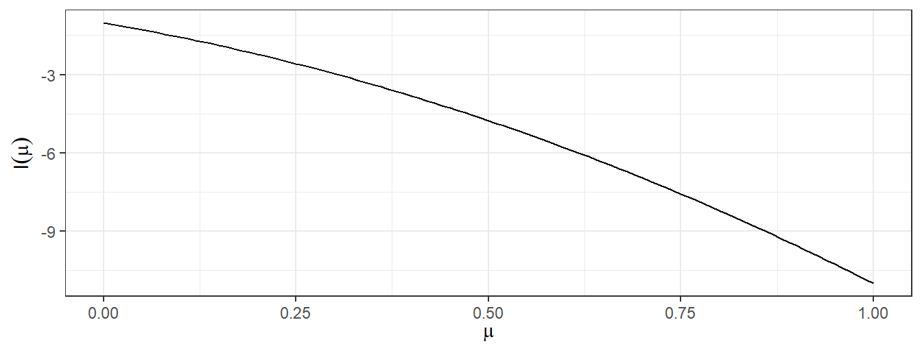
Figure 2.1: Log likelihood function for normal model with MLE on the boundary

With \(\overline{x}<0\) the log likelihood is larger at \(\mu=0\) than for any \(\mu>0,\) so that the MLE is then \(\hat{\mu}=0,\) yet this is not a stationary point of the log likelihood function.

2.2.1 Multivariate case

We now consider the case where the parameter is multivariate \(\theta=(\theta_{1}, \ldots,\theta_{p}).\) We seek the value of \(\theta\) which maximises \(L(\theta \, | \, \mathbf x)=L(\theta_{1}, \ldots,\theta_{p} \, | \, \mathbf x),\) or equivalently the log likelihood function. Candidate values for the MLE are those values of \(\theta\) for which the partial derivatives of the log likelihood are all zero: \[\begin{eqnarray*} \frac{\partial}{\partial \theta_{r}} l(\theta \, | \, \mathbf{x}) & = & 0 \end{eqnarray*}\] for each \(r=1, \ldots, p\).

For such values of \(\theta,\) a sufficient condition for them to be a (local) maximum is that the Hessian matrix of the log likelihood is a negative definite matrix. The Hessian matrix is given by

\[\begin{eqnarray*} H(\theta) = \begin{pmatrix} \frac{\partial^{2}}{\partial \theta_{1}^{2}} l(\theta \, | \, \mathbf{x}) & \frac{\partial^{2}}{\partial \theta_{1} \partial \theta_{2}} l(\theta \, | \, \mathbf{x}) & \dots & \frac{\partial^{2}}{\partial \theta_{1} \partial \theta_{p}} l(\theta \, | \, \mathbf{x}) \\ \frac{\partial^{2}}{\partial \theta_{2} \partial \theta_{1}} l(\theta \, | \, \mathbf{x}) & \frac{\partial^{2}}{\partial \theta_{2}^{2}} l(\theta \, | \, \mathbf{x}) & \dots & \frac{\partial^{2}}{\partial \theta_{2} \partial \theta_{p}} l(\theta \, | \, \mathbf{x}) \\ \vdots & \vdots & \ddots & \vdots \\ \frac{\partial^{2}}{\partial \theta_{p} \partial \theta_{1}} l(\theta \, | \, \mathbf{x}) & \frac{\partial^{2}}{\partial \theta_{p} \partial \theta_{2}} l(\theta \, | \, \mathbf{x}) & \dots & \frac{\partial^{2}}{\partial \theta_{p}^{2}} l(\theta \, | \, \mathbf{x}) \end{pmatrix} \end{eqnarray*}\]

The matrix \(H(\theta)\) is negative definite at \(\hat{\theta}\) if for all non-zero vectors \(a=(a_{1}, \ldots,a_{p})^{T},\) \[\begin{eqnarray*} a^{T} H(\hat{\theta}) a < 0. \end{eqnarray*}\]

Example 2.7 (Normal distribution, mean and variance unknown) Suppose that \(X_{1}, \ldots,X_{n}\) are i.i.d. draws from \(N(\mu,\sigma^{2}),\) with now both \(\mu\) and \(\sigma^{2}\) unknown. Thus now \(\theta=(\mu,\sigma^{2}).\) We showed earlier (in Example 2.2) that the log likelihood is given by \[\begin{eqnarray*} l(\theta \, | \, \mathbf{x}) & = & - \frac{n}{2}\log(2\pi \sigma^{2}) - \frac{1}{2\sigma^{2}} \sum^{n}_{i=1} (x_{i}-\mu)^{2}. \end{eqnarray*}\] The first order partial derivatives are \[\begin{eqnarray*} \frac{\partial l}{\partial \mu} & = & \frac{1}{\sigma^{2}} \sum_{i=1}^{n}(x_{i} - \mu); \\ \frac{\partial l}{\partial \sigma^{2}} & = & -\frac{n}{2\sigma^{2}} + \frac{1}{2(\sigma^{2})^{2}}\sum_{i=1}^{n}(x_{i} - \mu)^{2}. \end{eqnarray*}\] Solving \(\frac{\partial l}{\partial \mu} = 0\) we find that, for \(\sigma^{2} > 0,\) \(\hat{\mu} = \frac{1}{n} \sum_{i=1}^{n} x_{i} = \overline{x}.\) Substituting this into \(\frac{\partial l}{\partial \sigma^{2}} = 0\) gives \[\begin{eqnarray*} -\frac{n}{2\sigma^{2}} + \frac{1}{2(\sigma^{2})^{2}}\sum_{i=1}^{n}(x_{i} - \overline{x})^{2} & = & 0, \end{eqnarray*}\] so that \(\hat{\sigma}^{2} = \frac{1}{n} \sum_{i=1}^{n} (x_{i} - \overline{x})^{2}.\) The second order partial derivatives are \[\begin{eqnarray*} \frac{\partial^{2} l}{\partial \mu^{2}} & = & -\frac{n}{\sigma^{2}}; \\ \frac{\partial^{2} l}{\partial (\sigma^{2})^{2}} & = & \frac{n}{2(\sigma^{2})^{2}} - \frac{1}{(\sigma^{2})^{3}}\sum_{i=1}^{n}(x_{i} - \mu)^{2}; \\ \frac{\partial^{2} l}{\partial \mu \partial \sigma^{2}} & = & - \frac{1}{(\sigma^{2})^{2}}\sum_{i=1}^{n}(x_{i} - \mu) \ = \ \frac{\partial^{2} l}{\partial \sigma^{2} \partial \mu}. \end{eqnarray*}\] Evaluating these at \(\hat{\mu} = \overline{x},\) \(\hat{\sigma}^{2} = \frac{1}{n} \sum_{i=1}^{n} (x_{i} - \overline{x})^{2}\) gives \[\begin{eqnarray*} \left.\frac{\partial^{2} l}{\partial \mu^{2}}\, \right|_{\mu = \hat{\mu}, \sigma^{2} = \hat{\sigma}^{2}}& = & -\frac{n}{\hat{\sigma}^{2}}; \\ \left.\frac{\partial^{2} l}{\partial (\sigma^{2})^{2}}\right|_{\mu = \hat{\mu}, \sigma^{2}= \hat{\sigma}^{2}} & = & \frac{n}{2(\hat{\sigma}^{2})^{2}} - \frac{1}{(\hat{\sigma}^{2})^{3}}\sum_{i=1}^{n}(x_{i} - \overline{x})^{2} \ = \ -\frac{n}{2(\hat{\sigma}^{2})^{2}}; \\ \left.\frac{\partial^{2} l}{\partial \mu \partial \sigma^{2}}\right|_{\mu = \hat{\mu}, \sigma^{2}= \hat{\sigma}^{2}} & = & - \frac{1}{(\hat{\sigma}^{2})^{2}}\sum_{i=1}^{n}(x_{i} - \overline{x}) \ = \ 0. \end{eqnarray*}\] A sufficient condition for \(L(\hat{\mu}, \hat{\sigma}^{2} \, | \, \mathbf{x})\) to be a maximum is that the matrix \[\begin{eqnarray*} H(\hat{\theta}) \ = \ \left.\left(\begin{array}{cc} \frac{\partial^{2} l}{\partial \mu^{2}} & \frac{\partial^{2} l}{\partial \mu \partial \sigma^{2}} \\ \frac{\partial^{2} l}{\partial \sigma^{2} \partial \mu} & \frac{\partial^{2} l}{\partial (\sigma^{2})^{2}} \end{array} \right)\right|_{\mu = \hat{\mu}, \sigma^{2}= \hat{\sigma}^{2}} \ = \ \left(\begin{array}{cc} -\frac{n}{\hat{\sigma}^{2}} & 0 \\ 0 & -\frac{n}{2(\hat{\sigma}^{2})^{2}} \end{array} \right) \end{eqnarray*}\] is negative definite. For any non-zero vector \(a = (a_{1},a_{2})^{T}\) we have \[\begin{eqnarray*} a^{T} H(\hat{\theta}) a & = & -\frac{na_{1}^{2}}{\hat{\sigma}^{2}} - \frac{na_{2}^{2}}{2(\hat{\sigma}^{2})^{2}} < 0 \end{eqnarray*}\] so that \(H(\hat{\theta})\) is negative definite. The maximum likelihood estimates are \(\hat{\mu} = \overline{x}\) and \(\hat{\sigma}^{2} = \frac{1}{n} \sum_{i=1}^{n} (x_{i} - \overline{x})^{2}.\) The corresponding maximum likelihood estimators are \(\overline{X}\) and \(\frac{1}{n} \sum_{i=1}^{n} (X_{i} - \overline{X})^{2}\) for \(\mu\) and \(\sigma^{2}\) respectively.

Example 2.8 Recall the NHANES BMI data from Example 1.7. We have data on 1,638 individuals between 20 and 39 years of age who had BMI recorded in the study. We are interested in estimating the population mean BMI \(\mu,\) and we do not know the population variance \(\sigma^{2}.\) Assuming the population distribution of BMIs is normal \(N(\mu,\sigma^{2}),\) we can obtain a point estimate for \(\mu\) using the MLE \(\hat{\mu}=\overline{x}= 27.9\). This is also the MOM estimate for \(\mu.\)

2.2.2 Invariance principle

Suppose that in addition to finding the MLE for \(\theta\) we are also interested in finding the MLE for some function, \(g(\theta)\), of \(\theta\). For example, if \(\theta\) is the variance then we might be interested in the precision, \(1/\theta\), or the standard deviation, \(\sqrt{\theta}\).

Maximum likelihood estimation enjoys the so called invariance principle in respect of transformation of the model parameters. Informally, if \(\hat{\theta}\) is the MLE of \(\theta\) then \(g(\hat{\theta})\) is the MLE of \(g(\theta)\). We now formalise this approach.

Let \(\theta\) denote the model parameters and consider a transformation of \(\theta,\) given by \(\psi=g(\theta).\) If the transformation is one-to-one (so each \(\theta\) corresponds to a unique value of \(g(\theta)\) and vice versa) then the likelihood function for \(\psi\) is given by \(L^{*}(\psi \, | \,\mathbf x)=L(g^{-1}(\psi) \, | \,\mathbf x)\). In the more general case, we make the following definition of the induced likelihood function of the transformed parameter.

Definition 2.4 (Induced likelihood of transformed parameter) Let \(\psi=g(\theta)\) be a transformation of the model parameter \(\theta.\) The induced likelihood function for the transformed parameter \(\psi\) is defined as \[\begin{eqnarray*} L^*(\psi \, | \, \mathbf x) = \underset{\{\theta : g(\theta)=\psi\}}{\mbox{sup}} L(\theta \, | \, \mathbf{x}). \end{eqnarray*}\]

Theorem 2.1 (Invariance principle for maximum likelihood estimator) Suppose that \(\hat{\theta}\) is the MLE of \(\theta.\) Then \(g(\hat{\theta})\) is the MLE of \(\psi=g(\theta).\)

Proof: If the transformation \(g(\theta)\) is one-to-one the result is clear. For the general case, see the proof of Theorem 7.2.10 in Casella and Berger. \(\Box\)

Example 2.9 (MLE of the standard deviation) In Example 2.7 we showed that the MLE of the variance in the normal model is \(\hat{\sigma}^{2}=\frac{1}{n} \sum_{i=1}^{n} (X_{i} - \overline{X})^{2}.\) By the invariance property, Theorem 2.1, we can immediately deduce that the MLE of the standard deviation is \(\hat{\sigma}=\sqrt{\frac{1}{n} \sum_{i=1}^{n} (X_{i} - \overline{X})^{2}}.\)

2.3 Evaluating point estimators

We have seen two approaches for deriving estimators. We now consider ways in which we can judge the quality of competing estimators. We do so by examining their so called frequentist properties, that is how they perform in (hypothetical) repeated samples from the population or repeated experiments.

2.3.1 Bias and variance

Definition 2.5 (Bias of an estimator) The bias of an estimator is defined as the difference between its expected value in repeated samples and the true parameter value: \[\begin{eqnarray*} \text{Bias}(\hat{\theta},\theta) & = & E(\hat{\theta}) - \theta. \end{eqnarray*}\]

Note that if there is no confusion about the parameter \(\theta\) being estimated then we may suppress the direct reference to \(\theta\) and write \(\text{Bias}(\hat{\theta})\). In general the bias could depend on the true parameter value \(\theta\), although as we shall see sometimes this is not the case. As we shall also see, the bias may depend on the sample size \(n\). If the bias is zero for all true parameter values, we say the estimator is unbiased.

Example 2.10 (Bias of sample mean) Suppose \(X_{1}, \ldots,X_{n}\) are i.i.d. from a distribution with mean \(\mu.\) Then the sample mean \(\hat{\mu} = \frac1n \sum X_{i}\) is unbiased, since \[\begin{eqnarray*} E(\hat{\mu}) & = & E\left(\frac1n \sum^{n}_{i=1} X_{i}\right) \ = \ \frac1n \sum^{n}_{i=1} E(X_{i}) \\ & = & \frac1n n \mu \ = \ \mu. \end{eqnarray*}\]

Assuming our estimator is unbiased or has small bias, we would like our estimator to have small variance, since small variance means that the estimator on average is close (in squared distance) to its mean.

Example 2.11 (Variance of sample mean) Suppose \(X_{1}, \ldots,X_{n}\) are i.i.d. from a distribution with mean \(\mu\) and finite variance \(\sigma^{2}.\) Then the variance of the sample mean is given by \[\begin{eqnarray*} \text{Var}(\hat{\mu}) & = & \text{Var}\left( \frac1n \sum^{n}_{i=1} X_{i} \right) = \frac1{n^2} \sum^{n}_{i=1} \text{Var}(X_{i}) \\ & = & \frac1{n^2} n \sigma^{2} = \frac1n \sigma^{2}. \end{eqnarray*}\]

Putting Examples 2.10 and 2.11 together, we have that:

• The sample mean is unbiased for the true mean \(\mu.\)

• The variance of the sample mean decreases, like \(1/n\), as the sample size \(n\) increases.

Intuitively this makes sense - as the sample size \(n\) increases, the estimate will tend to be closer on average to the true mean.

Definition 2.6 (Standard error) The standard error of an estimator \(\hat{\theta}\) is defined as \(\sqrt{\text{Var}(\hat{\theta})}.\)

Example 2.12 (Standard error of sample mean) Following on from Example 2.11, the standard error of the sample mean is given by \[\begin{eqnarray*} \sqrt{\text{Var}(\hat{\mu})} & = & \frac{1}{\sqrt{n}} \sigma. \end{eqnarray*}\] Thus, for example, reducing the error in the estimate of \(\mu\) by a factor of two would take four times as many sample observations.

We now consider an estimator which, unlike the sample mean, is not unbiased (for finite \(n\)).

Example 2.13 (Bias of method of moments variance estimator) Consider again the method of moments estimator of the variance \(\hat{\sigma}^{2}=\frac1n \sum (X_{i}-\hat{\mu})^2\) where \(\hat{\mu} = \overline{X}\). We have \[\begin{eqnarray*} E\left(\frac{1}{n} \sum^{n}_{i=1} (X_{i}-\overline{X})^2 \right) & = & \frac{1}{n} \sum_{i=1}^{n} \text{Var} (X_{i} - \overline{X}) \\ & = & \frac{1}{n} \sum_{i=1}^{n} \left\{\text{Var}(X_{i}) - 2\text{Cov}(X_{i}, \overline{X})+\text{Var}(\overline{X})\right\} \\ & = & \frac{1}{n}\sum_{i=1}^{n} \left\{\sigma^{2} - 2\text{Cov}(X_{i}, \overline{X}) + \frac{\sigma^{2}}{n}\right\}. \end{eqnarray*}\] Now, noting that \(\text{Var}(X_{i}) = \text{Cov}(X_{i}, X_{i})\), \[\begin{eqnarray*} \text{Cov}(X_{i}, \overline{X}) & = & \frac{1}{n} \sum_{j=1}^{n} \text{Cov}(X_{i}, X_{j}) \\ & = & \frac{1}{n} \left\{\text{Var}(X_{i}) + \sum_{j \neq i}^{n} \text{Cov}(X_{i}, X_{j}) \right\} \\ & = & \frac{1}{n} \left\{\sigma^{2} + \sum_{j \neq i}^{n} 0 \right\} \\ & = & \frac{\sigma^{2}}{n} \end{eqnarray*}\] since the \(X_{i}\)s are independent. Consequently, \[\begin{eqnarray} E\left(\frac1n \sum^{n}_{i=1} (X_{i}-\overline{X})^2 \right) & = & \frac{1}{n} \sum_{i=1}^{n}\left\{\sigma^{2} -2\frac{\sigma^{2}}{n} + \frac{\sigma^{2}}{n}\right\} \\ & = & \frac{(n-1)}{n}\sigma^{2}. \tag{2.1} \end{eqnarray}\] The method of moments variance estimator is thus biased downwards by \(\sigma^{2}/n.\) Note that, by multiplying Equation (2.1) by \(n/(n-1)\), we have that the estimator \[\begin{eqnarray*} S^{2} & = & \frac{1}{n-1} \sum_{i=1}^{n} (X_{i}-\overline{X})^{2}. \end{eqnarray*}\] is an unbiased estimator of the population variance.

Note that the (absolute) bias of \(\hat{\sigma}^{2}\) depends on the true parameter value of \(\sigma^{2}\). From Equation (2.1), we can also see that the bias tends to zero as \(n\rightarrow \infty.\) It is thus asymptotically unbiased. It turns out that quite a lot of the most used statistical methods are biased for finite sample sizes and only unbiased asymptotically (in the limit).

2.3.2 Mean squared error

Bias is just one facet of an estimator. Consider the following two scenarios.

1. The estimator \(\hat{\theta} = \hat{\theta}(X_{1}, \ldots, X_{n})\) may be unbiased but the sampling distribution, \(f(\hat{\theta} \ | \ \theta)\), may be quite disperse: there is a large probability of being far away from \(\theta\), so for any \(\epsilon > 0\) the probability that \(P(\theta - \epsilon < \hat{\theta} < \theta + \epsilon)\) is small.

2. The estimator \(\hat{\theta}\) may be biased but the sampling distribution, \(f(\hat{\theta} \, | \, \theta)\), may be quite concentrated. So, for any \(\epsilon > 0\) the probability that \(P(\theta - \epsilon < \hat{\theta} < \theta + \epsilon )\) is large.

In these cases, the biased estimator may be preferable to the unbiased one. We would like to know more than whether or not an estimator is biased. In particular, we wish to capture some idea of how concentrated the sampling distribution of the estimator \(\hat{\theta}\) is around \(\theta\). Ideally we would like \[\begin{eqnarray*} P(|\hat{\theta} - \theta| < \epsilon) & = & P(\theta - \epsilon < \hat{\theta} < \theta + \epsilon) \end{eqnarray*}\] to be large for all \(\epsilon > 0\). This probability may be hard to evaluate, but we may make use of Chebyshev’s inequality.

Theorem 2.2 (Chebyshev's inequality) Let \(Y\) be a random variable with finite mean \(\mu\) and finite variance \(\sigma^{2}.\) For any \(\epsilon>0\) and \(c \in \mathbb{R}\) \[\begin{eqnarray*} P(|Y - c| \geq \epsilon) \leq \frac{E\{(Y-c)^{2}\}}{\epsilon^{2}} \end{eqnarray*}\] so that \(P(|Y - c| < \epsilon) \geq 1 - \frac{E\{(Y-c)^{2}\}}{\epsilon^{2}}\).

Proof: (For completeness; non-examinable) Suppose that \(Y\) is continuous (the result holds more generally than this), and let the density of \(Z=Y-c\) be \(f(z).\) Then \[\begin{eqnarray*} E(Z^{2}) & = & \int z^{2} f(z) dz \\ & = &\int_{|z|\geq \epsilon} z^{2} f(z) dz + \int_{|z|<\epsilon} z^{2} f(z) dz \\ & \geq & \int_{|z|\geq \epsilon} z^{2} f(z) dz \\ & \geq & \epsilon^{2} \int_{|z|\geq \epsilon} f(z) dz = \epsilon^{2} P(|Z| \geq \epsilon). \end{eqnarray*}\] The result then follows by rearrangement. \(\Box\)

A common choice of \(c\) is \(E(Y)\) so that \[\begin{eqnarray*} P(|Y - E(Y)| \geq \epsilon) \leq \frac{Var(Y)}{\epsilon^{2}}. \end{eqnarray*}\] For an estimator \(\hat{\theta}\) we are interested in \(|\hat{\theta} - \theta|\) (which reduces to \(|\hat{\theta} - E(\hat{\theta})|\) in the case when \(\hat{\theta}\) is an unbiased estimator of \(\theta\)) and so applying Chebyshev’s inequality with \(Y = \hat{\theta}\) and \(c = \theta\) gives \[\begin{eqnarray*} P(|\hat{\theta} - \theta| < \epsilon) & \geq & 1 - \frac{E\{(\hat{\theta} - \theta)^{2}\}}{\epsilon^{2}}. \end{eqnarray*}\] Consequently, we will be interested in estimators for which \(E\{(\hat{\theta} - \theta)^{2}\}\), the average distance between the estimator and its target parameter, is small. This quantity is formally known as the mean squared error (MSE).

Definition 2.7 (Mean squared error) The mean squared error of an estimator \(\hat{\theta}\) is defined as \[\begin{eqnarray*} \text{MSE}(\hat{\theta},\theta) & = & E\left\{(\hat{\theta} - \theta)^{2}\right\}. \end{eqnarray*}\]

Note that if there is no confusion about the parameter \(\theta\) being estimated then we may suppress the direct reference to \(\theta\) and write \(\text{MSE}(\hat{\theta})\). We now show that the MSE is equal to the sum of the squared bias and variance.

Theorem 2.3 The mean squared error of an estimator \(\hat{\theta}\) can be expressed as \[\begin{eqnarray*} \text{MSE}(\hat{\theta},\theta) & = & \text{Var}(\hat{\theta}) + \text{Bias}(\hat{\theta},\theta)^{2}. \end{eqnarray*}\]

Proof: \[\begin{eqnarray*} \text{MSE}(\hat{\theta},\theta) & = & E\left[(\hat{\theta}-\theta)^2\right]\\ & = & E\left[\left(\hat{\theta}-E[\hat{\theta}]-(\theta-E[\hat{\theta}])\right)^2\right]\\ & = & E\left[\left(\hat{\theta}-E[\hat{\theta}]\right)^2\right]+E\left[\left(\theta-E[\hat{\theta}]\right)^2\right]-2\,(\theta-E[\hat{\theta}])E\left[\hat{\theta}-E[\hat{\theta}]\right] \\ & = & E\left[\left(\hat{\theta}-E[\hat{\theta}]\right)^2\right]+E\left[\left(\theta-E[\hat{\theta}]\right)^2\right]\\ & = & \text{Var}[\hat{\theta}]+\left(E[\hat{\theta}]-\theta\right)^2\\ \end{eqnarray*}\] since \(E\left[\hat{\theta}-E[\hat{\theta}]\right]\) is zero and \(E[\hat{\theta}]-\theta\) is a constant. \(\Box\)

If we have a choice between estimators then we might prefer to use the estimator with the smallest MSE.

Definition 2.8 (Relative Efficiency) Suppose that \(T_{1} = T_{1}(X_{1}, \ldots, X_{n})\) and \(T_{2} = T_{2}(X_{1}, \ldots, X_{n})\) are two estimators for \(\theta.\) The efficiency of \(T_{1}\) relative to \(T_{2}\) is \[\begin{eqnarray*} \mbox{RelEff}(T_{1}, T_{2},\theta) & = & \frac{\text{MSE}(T_{2},\theta)}{\text{MSE}(T_{1},\theta)}. \end{eqnarray*}\]

Hopefully \(\mbox{RelEff}(T_{1}, T_{2},\theta)\) does not depend on the true unknown \(\theta,\) in which case we simply write \(\mbox{RelEff}(T_{1}, T_{2}).\) Values of \(\mbox{RelEff}(T_{1}, T_{2})\) less than 1 then suggest a preference for the estimator \(T_{2}\) over \(T_{1}\) while values greater than 1 of \(\mbox{RelEff}(T_{1}, T_{2})\) suggest a preference for \(T_{1}.\) Notice that if \(T_{1}\) and \(T_{2}\) are unbiased estimators then \[\begin{eqnarray*} \mbox{RelEff}(T_{1}, T_{2}, \theta) & = & \frac{\text{Var}(T_{2})}{\text{Var}(T_{1})}, \end{eqnarray*}\] and we choose the estimator with the smallest variance.

We now consider two examples.

Example 2.14 (Two estimators of the mean of a normal distribution) In Examples 2.10 and 2.11 we showedthat the sample mean, \(\overline{X}\), is unbiased and has variance \(\sigma^2/n.\) Suppose that \(X_{1}, \ldots,X_{n}\) are i.i.d. from \(N(\mu,\sigma^{2}).\) Then since for the normal the mean and median are identical, an alternative estimator for \(\mu\) is the sample median, \(\text{med}\{X_{1}, \ldots, X_{n}\}\). It turns out that for the normal distribution, and with large \(n,\) the sample median is approximately normally distributed with mean \(\mu\) and variance \(\pi \sigma^{2} / (2n).\) The relative efficiency of \(T_{1}=\overline{X}\) and \(T_{2} = \text{med}\{X_{1}, \ldots, X_{n}\}\) is thus \[\begin{eqnarray*} \mbox{RelEff}(T_{1}, T_{2}) & = &\frac{\pi \sigma^{2} / (2n)}{\sigma^{2}/n} = \pi/2. \end{eqnarray*}\] Thus under the normal model, we would prefer \(\overline{X}\) for estimating \(\mu\) to the sample median.

In the next example we will consider the relative efficiency of two alternative estimators for the variance \(\sigma^{2}\) in the normal \(N(\mu,\sigma^{2})\) model. These are:

• the unbiased sample variance \(S^{2}=\frac{1}{(n-1)}\sum^{n}_{i=1}(X_{i}-\overline{X})^{2}\)

• the biased method of moments estimator \(\hat{\sigma}^{2} = \frac{1}{n}\sum^{n}_{i=1}(X_{i}-\overline{X})^{2}.\)

To proceed we will need the variance of both \(S^{2}\) and \(\hat{\sigma}^{2}\). In Section 3.2, as a consequence of Theorem 3.1, we will demonstrate that \[\begin{eqnarray*} Var(S^{2}) & = & \frac{2\sigma^{4}}{n-1}. \end{eqnarray*}\] Noting that \[\begin{eqnarray*} \hat{\sigma}^{2} \ = \ \frac{1}{n}\sum^{n}_{i=1}(X_{i}-\overline{X})^{2} \ = \ \frac{n-1}{n} S^{2} \end{eqnarray*}\] it follows that \[\begin{eqnarray*} \text{Var}(\hat{\sigma}^{2}) & = & \text{Var}\left[\frac{n-1}{n} S^{2} \right] \\ & = & \frac{(n-1)^{2}}{n^{2}} \text{Var}(S^{2}) \\ & = & \frac{(n-1)^{2}}{n^{2}} \frac{2 \sigma^{4}}{n-1} = \frac{2(n-1)\sigma^{4}}{n^{2}}. \end{eqnarray*}\] We are now in a position to calculate the relative efficiency of the two estimators.

Example 2.15 (Two estimators of the variance of a normal distribution) Suppose that \(X_{1}, \ldots, X_{n}\) are i.i.d. \(N(\mu, \sigma^{2}).\) From Example 2.13, \(T_{1} = \hat{\sigma}^{2} = \frac{1}{n} \sum_{i=1}^{n} (X_{i} - \overline{X})^{2}\) is a biased estimator of \(\sigma^{2}\) with \[\begin{eqnarray*} \text{Bias}(T_{1}) & = & (1-n^{-1})\sigma^{2} - \sigma^{2} = -\frac{\sigma^{2}}{n}. \end{eqnarray*}\] Hence, \[\begin{eqnarray*} \text{MSE}(T_{1}) & = & Var(T_{1}) + \text{Bias}(T_{1})^{2} \\ & = & \frac{2(n-1)\sigma^{4}}{n^{2}} + \frac{\sigma^{4}}{n^{2}} = \frac{(2n-1)\sigma^{4}}{n^{2}}. \end{eqnarray*}\] An unbiased estimator of \(\sigma^{2}\) is \(T_{2} =S^2= \frac{1}{n-1} \sum_{i=1}^{n} (X_{i} - \overline{X})^{2}\). Thus, \(\text{MSE}(T_{2}) = \text{Var}(T_{2}) = 2\sigma^{4}/(n-1).\) Hence, the relative efficiency of \(T_{1}\) to \(T_{2}\) is \[\begin{eqnarray*} \mbox{RelEff}(T_{1}, T_{2}) & = & \frac{\text{MSE}(T_{2})}{\text{MSE}(T_{1})} \\ & = & \frac{2\sigma^{4}/(n-1)}{(2n-1)\sigma^{4}/n^{2}} \\ & = & \frac{2n^{2}}{(2n-1)(n-1)} > 1 \ \mbox{if $n > 1/3$}. \end{eqnarray*}\] Although \(T_{1}\) is biased, it is more concentrated around \(\sigma^{2}\) than \(T_{2}.\)

2.3.3 Convergence in probability and consistency

Bias and MSE are criteria for a fixed sample size \(n\). We might also be interested in large sample properties. Let \(T_{n} = T_{n}(X_{1}, \ldots, X_{n})\) be an estimator for \(\theta\) based on a sample of size \(n\), \(X_{1}, \ldots, X_{n}\). What can we say about \(T_{n}\) as \(n \rightarrow \infty?\) It might be desirable if, roughly speaking, the larger \(n\) is, the ‘closer’ \(T_{n}\) is to \(\theta\).

The behaviour of estimators when the sample size increases to infinity is referred to as the asymptotic behaviour. Whilst we will never have an infinite amount of data in reality, we might consider asymptotic results as approximations to the finite \(n\) behaviour, always mindful however that the approximation may not necessarily be good.

Definition 2.9 (Convergence in probability) A sequence of random variables \((A_{n})_{n \in \mathbb{N}} = (A_{1}, A_{2}, \ldots)\) is said to converge in probability to a random variable \(A,\) denoted \(A_{n} \xrightarrow{P} A\), if for every \(\epsilon>0\) \[\begin{eqnarray} P(|A_{n}-A|<\epsilon) \rightarrow 1 \text{ as } n \rightarrow \infty. \tag{2.2} \end{eqnarray}\]

Note that an equivalent condition to (2.2) is that \[\begin{eqnarray*} P(|A_{n}-A| \geq \epsilon) \rightarrow 0 \text{ as } n \rightarrow \infty. \end{eqnarray*}\]

By considering the random variable \(A\) with distribution \(P(A = c) = 1\), Definition 2.9 includes the case where the limiting random variable, \(A\), is a constant, \(c\). This will be useful for our purposes: in estimation problems it is desirable for the sequence of estimators of a parameter to converge in probability to the parameter.

Definition 2.10 (Consistent estimator) An estimator \(T_{n}=T_{n}(X_{1}, \ldots,X_{n})\) is consistent for the parameter \(\theta\) if the sequence \((T_{n})_{n \in \mathbb{N}}\) satisfies \(T_{n} \xrightarrow{P} \theta\) for every \(\theta \in \Theta\).

Thus, an estimator is consistent if it is possible to get arbitrarily close to \(\theta\) by taking the sample size \(n\) sufficiently large. Now, from Chebyshev’s inequality, Theorem 2.2, we have a lower bound for \(P(|T_{n} - \theta| < \epsilon)\), while 1 is an upper bound, so that \[\begin{eqnarray*} 1 \ \geq \ P(|T_{n} - \theta| < \epsilon) \ \geq 1 - \frac{MSE(T_{n})}{\epsilon^{2}}. \end{eqnarray*}\]
Hence, a sufficient condition for consistency of the estimator \(T_{n}\) is that \[\begin{eqnarray*} \lim_{n \rightarrow \infty} MSE(T_{n}) & = & 0. \end{eqnarray*}\] As \(MSE(T_{n}) = Var(T_{n})+\text{Bias}(T_{n})^{2}\) then a sufficient condition that \(\lim_{n \rightarrow \infty} MSE(T_{n}) = 0\), and thus for consistency, is that both \[\begin{eqnarray*} \lim_{n \rightarrow \infty} \text{Bias}(T_{n}) = 0 & \text{ and } & \lim_{n \rightarrow \infty} \text{Var}(T_{n}) = 0. \end{eqnarray*}\]

Example 2.16 (Consistency of method of moments and MLE variance estimators for the normal) Suppose \(X_{1}, \ldots,X_{n}\) are i.i.d. \(N(\mu,\sigma^{2}).\) We previously showed that for \(T_{1} = \hat{\sigma}^{2} = \frac{1}{n} \sum_{i=1}^{n} (X_{i} - \overline{X})^{2}\): \[\begin{eqnarray*} \text{Bias}(T_{1}) = -\frac{\sigma^{2}}{n}; & & \text{Var}(T_{1}) = \frac{2(n-1)\sigma^{4}}{n^{2}}. \end{eqnarray*}\] Since both of these tend to zero as \(n \rightarrow \infty,\) it follows that \(T_{1}\) is consistent for \(\sigma^{2}.\) For the \(S^{2},\) we previously showed \(S^{2}\) is unbiased and also has variance which goes to zero as \(n \rightarrow \infty,\) so \(S^2\) is also consistent for \(\sigma^{2}.\)

Proposition 2.1 (Consistency of sample mean, weak law of large numbers) Suppose \(X_{1}, \ldots,X_{n}\) are i.i.d. with mean \(\mu\) and finite variance \(\sigma^{2}.\) Then \(\overline{X}_{n} = \frac{1}{n} \sum_{i=1}^{n} X_{i}\) is a consistent estimator for \(\mu.\)

Proof: We showed in Example 2.10 that the sample mean \(\overline{X}_{n}\) is unbiased for \(\mu.\) In Example 2.11 we showed it has variance \(\sigma^{2}/n.\) Let \((\overline{X}_{n})_{n \in \mathbb{N}}\) denote the corresponding sequence of estimators. Since the bias is zero, and the variance tends to zero as \(n \rightarrow \infty,\) it follows that the mean squared error of \(\overline{X}_{n}\) goes to zero as \(n \rightarrow \infty.\) Thus \(\overline{X}_{n} \xrightarrow{P} \mu.\) \(\square\)

Next we will show that the MLE in the exponential model is consistent. To do this, we first state an important theorem concerning the limit preserving features of continuous maps.

Theorem 2.4 (Continuous Mapping Theorem) Suppose the sequence of random variables \((A_{n})_{n \in \mathbb{N}} = (A_{1}, A_{2}, \ldots)\) are such that \(A_{n} \xrightarrow{P} A,\) and that \(g(\cdot)\) is a continuous function. Then \(g(A_{n}) \xrightarrow{P} g(A).\)

Proof: (Non-examinable) If \(g(\cdot)\) is continuous then given \(\epsilon > 0\) there exists a \(\delta > 0\) such that \(|a_{n} - a| < \delta\) implies \(|g(a_{n}) - g(a)| < \epsilon\). Consequently, \[\begin{eqnarray*} P(|g(A_{n}) - g(A)| < \epsilon) & \geq & P(|A_{n} - A| < \delta). \end{eqnarray*}\] From Definition 2.9, for every \(\delta\), \(P(|A_{n}-A|<\delta) \rightarrow 1\) as \(n \rightarrow \infty\). Thus, \(P(|g(A_{n}) - g(A)| < \epsilon) \rightarrow 1\) as \(n \rightarrow \infty\). As the choice of \(\epsilon\) was arbitrary, this must hold for every \(\epsilon > 0\). \(\Box\)

Example 2.17 (Consistency of MLE in the exponential model) Recall from Example 2.3 that the maximum likelihood estimator for \(\lambda\) in the exponential model is \(1/\overline{x}.\) For the exponential distribution, \(E(X)=\lambda^{-1}\) and \(\text{Var}(X)=\lambda^{-2}<\infty,\) so by the weak law of large numbers \(\overline{X}_{n} \xrightarrow{P} \lambda^{-1}.\) Since \(g(x)=x^{-1}\) is continuous, by Theorem 2.4 it then follows that \[\begin{eqnarray*} \hat{\lambda} & = & \frac{1}{\overline{X}} \xrightarrow{P} \frac{1}{\lambda^{-1}} = \lambda. \end{eqnarray*}\] Thus the MLE is consistent (although not unbiased) for \(\lambda.\)

2.4 Robustness to model misspecification

Up to now we have reasoned under the assumption that our posited parametric model is correctly specified. By this, we mean that the true data generating distribution belongs to the class of densities characterised by our model. As we will see in Chapter 5.4.2, it is possible to develop diagnostics and statistical tests to assess whether various model assumptions are reasonable in light of the observed data. Nevertheless, these have certain limitations, and so it is desirable that, if possible, our inferences are robust to certain model misspecifications.

A number of the estimators we have already seen are robust to misspecification, in the sense that properties such as unbiasedness and consistency are retained even if we relax some of the modelling assumptions. For example, it follows from Proposition 2.1 that the consistency of the method of moments and MLE \(\hat{\mu}\) in the normal model is robust to violations of the normality assumption.

Example 2.18 Recall the histogram Figure 1.1 of BMI values from the NHANES study. The histogram suggests a normality asssumption for the population distribution of BMI values is questionable. Nevertheless, in terms of point estimation for the mean \(\mu,\) we know from the preceding results that the MLE for the mean, which for the normal model is simply the sample mean, remains consistent for the population mean even if the population distribution of BMI values is not normal.

In Example 2.16 we proved that both \(T_{1}\) and \(S^{2}\) are consistent for \(\sigma^{2}\) under the normal model. The normal model was used to derive expressions for the variance of these two estimators, which we then saw tended to zero as \(n \rightarrow \infty.\) In practice the normality assumption might not hold. In this case, can we give similar guarantees about consistency of \(T_{1}\) and \(S^{2}\)? Before pursuing this further, we describe a further theorem which strengthens our ability to prove consistency.

Theorem 2.5 Let \(A_{n}\) and \(B_{n}\) denote sequences of random variables with \(A_{n} \xrightarrow{P} a\) and \(B_{n} \xrightarrow{P} b.\) Then \[\begin{eqnarray*} A_{n} + B_{n} & \xrightarrow{P} & a+b; \\ A_{n}B_{n} & \xrightarrow{P} & ab; \\ \text{ and} \quad \frac{A_{n}}{B_{n}} & \xrightarrow{P} & \frac{a}{b} \mbox{ provided } b \neq 0. \end{eqnarray*}\]

Proof: Omitted. See Chapter 2 of Lehmann if you are interested. \(\Box\)

We are now in a position to prove that both \(T_{1}\) and \(S^{2}\) are consistent for \(\sigma^{2}\) without the normality assumption.

Proposition 2.2 Let \(X_{1}, \ldots,X_{n}\) be i.i.d. with \(E(X^4)< \infty.\) Then \(T_{1}\) and \(S^{2}\) are both consistent estimators of \(\sigma^{2}.\) Furthermore, \(\sqrt{T_{1}}\) and \(S\) are consistent estimators of \(\sigma.\)

Proof: We first show that \(T_{1}\) is consistent for \(\sigma^{2},\) now without making any further distributional assumptions. We can express \(T_{1}\) as \[\begin{eqnarray*} T_{1} = \frac{1}{n} \sum_{i=1}^{n} (X_{i} - \overline{X})^{2} = \left[ \frac{1}{n} \sum_{i=1}^{n} X^{2}_{i} \right] - \overline{X}^{2}. \end{eqnarray*}\] By the weak law of large numbers (applied to \(X^2\), requiring a finite 4th moment), the first term converges in probability to \(E(X^2).\) By the Continuous Mapping Theorem, \(\overline{X}^{2} \xrightarrow{P} \mu^{2}.\) By Theorem 2.5 it thus follows that \(T_{1} \xrightarrow{P} E(X^{2}) - \mu^{2} = \text{Var}(X).\) For \(S^{2},\) since \[\begin{eqnarray*} S^{2} = \frac{1}{n-1} \sum^{n}_{i=1} (X_{i} - \overline{X})^{2} =\frac{1}{1-1/n} T_{1} \end{eqnarray*}\] and \(\frac{1}{1-1/n} \rightarrow 1\) as \(n \rightarrow \infty,\) it follows that \(S^{2} \xrightarrow{P} 1 \times \sigma^{2}=\sigma^{2}.\) Moreover, by the Continuous Mapping Theorem, it follows that \(\sqrt{T_{1}} \xrightarrow{P} \sigma\) and \(S \xrightarrow{P} \sigma\) since the square root function is continuous. \(\square\)