Chapter 1 Statistical models and inference
In this chapter we give an overview of statistical models and statistical inference, and through doing so, an overview of what this unit will cover. The purpose of a statistical model is to capture the stochastic (random) behaviour of some phenomenon of interest. Statistical models are not usually mechanistic models for the process under investigation. More commonly, they are empirical models that describe the variation in the data in a way that helps us answer particular substantive questions of interest.
1.1 Statistical models
A statistical model is a family of distributions which we believe includes – or at least approximates – the true, unknown distribution from which the data were generated. We shall proceed by assuming that our statistical model can be expressed as a parametric model.
Definition 1.1 (Parametric model) A parametric model for a random variable \(X\) is the triple \(\mathcal{E} = \{\mathcal{X}, \Theta, f_{X}(x \, | \, \theta)\}\) where only the finite dimensional parameter \(\theta \in \Theta\) is unknown.
Thus, the model specifies the sample space \(\mathcal{X}\) of the quantity to be observed \(X\), the parameter space \(\Theta\), and a family of distributions, \(\mathcal{F}\) say, where \(f_{X}(x \, | \, \theta)\) is the distribution for \(X\) when \(\theta\) is the value of the parameter. In this general framework, both \(X\) and \(\theta\) may be multivariate and we use \(f_{X}\) to represent the density function irrespective of whether \(X\) is continuous or discrete. If it is discrete then \(f_{X}(x \, | \, \theta)\) gives the probability of an individual value \(x\). Where there is no confusion about the random variable we will suppress the explicit reference to it, writing \(f(x \, | \, \theta)\). Typically, \(\theta\) is continuous-valued.
Statistics has a somewhat confusing convention of sometimes using \(\theta\) as an argument to a function and other times using it to denote the fixed but unknown true value of the parameter. We will stick to this convention, but where useful for clarity, we will denote the true value of the parameter by \(\theta^{*}.\)
Where \(\theta\) is a vector, often only a subset of the parameters will be of interest, meaning that our substantive questions of interest can be translated into questions about the values of these parameters. The other parameters are called nuisance parameters, which are needed in order for the model to adequately capture the probabilistic structure of the data but otherwise are not related to our substantive questions.
1.1.1 Examples
Example 1.1 (Bernoulli model) Suppose that \(X \sim \text{Bernoulli}(p)\), so that \(\mathcal{X} = \{0, 1\}\) and \[\begin{eqnarray*} P(X = x \, | \, p) & = & p^{x}(1-p)^{1-x}. \end{eqnarray*}\] The parameter \(p \in [0, 1]\) is continuous.
Example 1.2 (Binomial model) Suppose that, for \(i = 1, \ldots, n\), \(X_{i} \sim \text{Bernoulli}(p)\) and that the \(X_{i}\)s are independent. Then the sum, \(Y=\sum^{n}_{i=1} X_{i}\) is binomially distributed, which we denote as \(Y \sim Bin(n, p)\), with \[\begin{eqnarray*} P(Y = y \, | \, p) & = & \binom{n}{y}p^{y}(1-p)^{n-y} \end{eqnarray*}\] for \(y \in \{0, 1, \ldots, n\}\).
Example 1.3 (Normal model, unknown mean, known variance) Suppose that \(X \sim N(\mu,\sigma^{2})\) where \(\mu\) is the unknown mean and \(\sigma^{2}>0\) is the known variance. Then \[\begin{eqnarray*} f(x \, | \, \mu) & = & \frac{1}{\sqrt{2\pi}\sigma} \exp\left\{-\frac{1}{2\sigma^{2}}(x-\mu)^{2}\right\} \end{eqnarray*}\] for all \(x \in (-\infty, \infty)\).
Example 1.4 (Normal model, unknown mean, unknown variance) Suppose instead that \(X \sim N(\mu,\sigma^{2})\) where both \(\mu\) and \(\sigma^{2}\) are unknown. In this case, the parameter \(\theta = (\mu, \sigma^{2})\) is bivariate. If, for example, we were interested only in the mean \(\mu\) then \(\sigma^{2}\) is a nuisance parameter.
Example 1.5 (Exponential model) This model is often used to measure lifetimes or waiting times and we write \(X \sim \text{Exp}(\lambda)\) if \[\begin{eqnarray*} f(x \, | \, \lambda) & = & \left\{\begin{array}{cl} \lambda \exp(-\lambda x) & x \geq 0 \\ 0 & \text{otherwise.} \end{array} \right. \end{eqnarray*}\] The exponential model thus has support on the non-negative real line. The parameter \(\lambda>0\) is called the rate parameter.
Example 1.6 (Normal linear regression model) For each unit in the population there exists a fixed vector of covariates \(x_{i}\) and an outcome \(Y_{i}.\) The normal linear regression model stipulates that \[\begin{eqnarray*} Y_{i} = \beta^{T} x_{i} + \epsilon_{i} \end{eqnarray*}\] where \(\beta\) is a column vector of unknown parameters (regression coefficients) and \(\epsilon_{i}\) is a \(N(0,\sigma^{2})\) error term. Such models are the main focus of MA20227 Statistics 2B.
Learning about the parameter \(\theta\), that is making inferences about it, will be the key issue of interest. Typically, we discuss how we can estimate \(\theta\) based upon an observed random sample \(x_{1}, \ldots, x_{n}\) of observations believed to come from the underlying distribution \(f(x \, | \, \theta)\). Thus, the random variables \(X_{1}, \ldots, X_{n}\) will be independent and identically distributed.
1.1.2 Motivating examples
We now give some motivating illustrative examples where some of these statistical models could potentially be used to draw inferences about the phenomenon in question. We will return to these examples later during the unit.
Example 1.7 (Mean body mass index in NHANES) The National Health and Nutrition Examination Survey (NHANES) is a long running program of studies whose aim is to assess the health and nutritional status of adults and children in the United States. The survey consists of a combination of interviews with participants, physical examinations and laboratory tests.
Here we focus on data from the 2003-2004 study. We focus specifically on data from those aged between 20 and 39 years of age when the survey was performed, for a total of \(n = 1,753\) individuals. Figure 1.1 shows a histogram of body mass index (BMI) values for the 1,638 individuals between 20 and 39 years of age who had BMI recorded in the study.
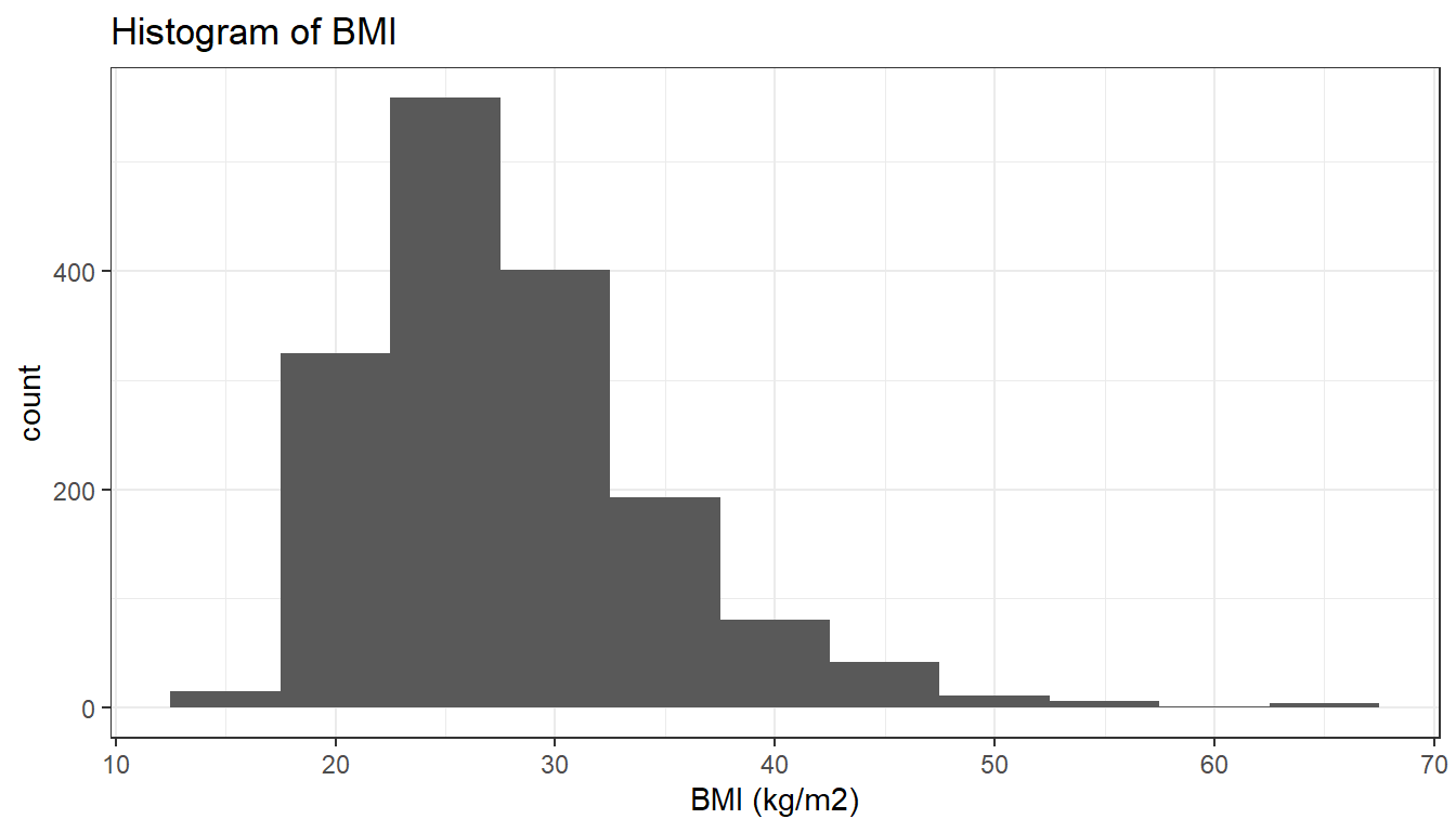
Figure 1.1: Histogram of 1,638 body mass index (kg/m2) values from NHANES 2003-2004
A statistical model we might use for the BMI data is to assume that the sample of BMI values are an i.i.d. sample from a \(N(\mu, \sigma^{2})\) distribution, and we are primarily interested in the population mean BMI \(\mu.\) The histogram shows a skewed distribution however, and so an initial concern is thus whether using a model which assumes a normal distribution is appropriate.
Note that the use of a statistical model here is to capture the randomness induced by the random sampling process. The BMI for each individual in the population is fixed at the time of the survey. However, the BMI values in our sample are modelled as random variables because, prior to the survey, we do not know which individuals will be selected into the sample.
Example 1.8 (Drinking in NHANES) The NHANES data introduced in the previous example contains many additional variables. A subset of these were based on asking participants about their consumption of alcohol. One of the questions asked was “In the past 12 months, on those days that you drank alcoholic beverages, on the average, how many drinks did you have?”. In order to learn about (reported) alcohol drinking behaviour, we will consider a dichotomised version of this variable, defined as whether they answered that they drank one drink on average on days they drank alcohol, or more than one.
For this variable \(n=1,104\) responded to the question, and of these, 846 (76.6%) answered that they drank more than one alcoholic drink on average on days that they did drink alcohol. Since each response is binary, we can use the i.i.d. Bernoulli model here, with the probability \(p\) representing the proportion of the population that would answer that they drink more than one alcoholic drink on average on days they drink.
Example 1.9 (Randomised two arm clinical trial in AIDS) The AIDS Clinical Trials Group Study 175 (ACTG175) was a randomised clinical trial conducted in the 1990s to compare different treatments for adults infected with HIV. We will focus on a comparison of those randomised to receive zidovudine treatment (532 patients) and those randomised to receive a combination treatment of zidovudine plus didanosine (522 patients). One of the outcomes is the patient’s CD4 blood cell count. A larger CD4 value is indicative that the treatment is working. Thus one of the analyses of interest is to compare the CD4 count after treatment with zidovudine plus didanosine compared to treatment with zidovudine alone. Figure 1.2 shows histograms of the CD4 count 20 weeks after baseline in these two groups.
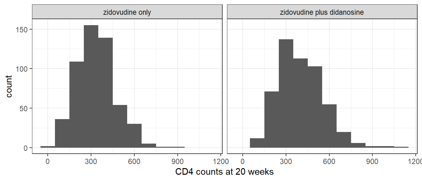
Figure 1.2: Histogram of CD4 T cell count at 20 weeks in zidovudine only versus zidovudine plus didanosine groups of ACTG175 trial
The comparison of these two treatment groups can be represented as a two-sample problem. In particular, our model will assume that the CD4 data on the patients in these two groups represent independent samples from the two hypothetical populations that would exist were we to treat all the eligible patients in the population with these two treatment options.
We let \(X_{1}, \ldots,X_{n_{0}}\) denote the patient’s CD4 counts in the zidovudine treatment group and \(Y_{1}, \ldots,Y_{n_{1}}\) the values in the zidovudine plus didanosine group. A possible parametric model is that \(X_{1}, \ldots,X_{n_{0}}\) are i.i.d. \(N(\mu_{X},\sigma^{2})\) and the \(Y_{1}, \ldots,Y_{n_{1}}\) are i.i.d. \(N(\mu_{Y},\sigma^{2}).\) This assumes the variance of CD4 count is the same in the two groups. A less restrictive (but still parametric) model would allow potentially distinct variances in the two groups. Primary interest could be in the contrast of \(\mu_{Y}\) with \(\mu_{X}.\) This is a so called two sample problem, which we will examine in Chapter 5.
Example 1.10 (Randomised two arm trial in cardiovascular disease) The Physician’s Health Study was an important medical study was carried out in the 1980s to investigate the benefit and risks of aspirin for cardiovascular disease and cancer. The trial randomised 22,071 healthy physicians to receive either aspirin or placebo. They were then followed-up to see which experienced heart attacks during the following 5 years. The data are shown in Table 1.1.
Table 1.1: Number of heart attacks by treatment group in the Physician’s Health Study Group Heart attack No heart attack Total Aspirin 139 10,898 11,037 Placebo 239 10,795 11,034 Primary interest is in whether receiving aspirin increases or decreases the probability of experiencing a heart attack. Let \(X_{i}\) denote the heart attack outcome (1=yes, 0=no) for the \(i\)th participant in the aspirin group, and \(Y_{i}\) denote the heart attack outcome in the \(i\)th participant in the placebo group. Then a natural model is to assume the \(X_{i}\) are i.i.d. Bernoulli with ‘success’ probability \(p_{X}\) and the \(Y_{i}\) are i.i.d. Bernoulli with ‘success’ probability \(p_{Y}.\) Primary interest could then be in the contrast of \(p_{X}\) with \(p_{Y}.\)
1.2 Statistical inference
The statistical inference problem is to make inferences about one or more parameters in the statistical model, based on the observed data. With a sample of infinite size, we would be able to empirically calculate the true parameter values of the model. In practice we observe data of finite size, meaning any estimates of the parameters will in general differ to some extent from their true values. The statistical inference problem then consists of a number of elements:
- What is our best guess or estimate of the unknown parameters based on the observed data? (point estimation, Chapter 2)
- How much uncertainty do we have in our parameter estimates? (confidence intervals, Chapter 3)
- Which of two competing hypotheses, specified in terms of model parameters, is true? (hypothesis testing, Chapter 4)
This unit will cover each of these steps in turn. At each step, we will also consider the robustness of our procedures to model misspecification. What guarantees, if any, can we have on the performance of our procedures if the true data generating distribution does not belong to the class of distributions characterised by our parametric model? Such robustness is desirable because, although the data can be used to some extent to check for model misspecification (see Section 5.4.2), it is impossible with a finite amount of data to prove a model is correctly specified.
In the final section of the unit (Chapter 5) we will apply our new skills from Chapters 2 – 4 to develop inferential techniques for investigating relationships between variables.