Chapter 3 Confidence intervals
A point estimate \(\hat{\theta}\) gives our best guess of the unknown parameter \(\theta\) based on the data. Unless we have very large samples, there will be some error in our estimates. In this chapter we introduce confidence intervals, which are used to communicate uncertainty in point estimates. Confidence intervals are random intervals that with a specified probability will include the true, unknown parameter value. They are useful to report along with point estimates to give an indication of how precise the point estimate is and to give a range of values of the unknown parameter that are plausible given the data.
3.1 Principles of confidence interval construction
We now consider construction of confidence intervals (CIs):
Definition 3.1 (Confidence interval) Let \(X_{1}, \ldots,X_{n}\) be a sample of data, and \(\theta\) denote an unknown parameter. Suppose that the random interval \[\begin{eqnarray*} \left(g_{1}(X_{1}, \ldots,X_{n}), g_{2}(X_{1}, \ldots,X_{n})\right) \end{eqnarray*}\] contains \(\theta\) with probability \(1-\alpha.\) Then we say that this interval is a \(100 \times (1-\alpha)\)% confidence interval for \(\theta,\) and has coverage level \(100 \times (1-\alpha)\)%. With observed data \(x_{1}, \ldots,x_{n},\) the realised value of this interval is \[\begin{eqnarray*} \left(g_{1}(x_{1}, \ldots,x_{n}), g_{2}(x_{1}, \ldots,x_{n})\right). \end{eqnarray*}\]
The next question is, how can we construct confidence intervals? One approach is based on a quantity known as a pivot.
Definition 3.2 (Pivot) Let \(X_{1}, \ldots,X_{n}\) be a random sample from \(f(x|\theta)\) with \(\theta\) unknown. A random variable \(\phi(X_{1}, \ldots,X_{n},\theta)\) is called a pivot if its distribution does not depend on \(\theta.\)
Example 3.1 Suppose that \(X_{1}, \ldots, X_{n}\) are i.i.d. \(N(\mu, \sigma^{2})\). There are (at most) two parameters: \(\mu\) and \(\sigma^{2}\). Note that, given \(\mu\) and \(\sigma^{2}\), \[\begin{eqnarray*} \frac{\overline{X} - \mu}{\sigma/\sqrt{n}} \sim N(0, 1) \end{eqnarray*}\] and \(N(0, 1)\) does not depend upon either \(\mu\) or \(\sigma^{2}\). Thus, \(\frac{\overline{X} - \mu}{\sigma/\sqrt{n}}\) is a pivot.
If we have a pivot then based on its known distribution, we find values \(c_{1}\) and \(c_{2}\) such that \[\begin{eqnarray*} P(c_{1} < \phi(X_{1}, \ldots,X_{n},\theta) < c_{2}) = 1-\alpha. \end{eqnarray*}\] The key idea here is that since the distribution of \(\phi(\cdot)\) does not depend on \(\theta\), the value \(c_1\) and \(c_2\) also do not depend on \(\theta\).
We then attempt to re-arrange the inequality so that \[\begin{eqnarray*} P\left(g_{1}(X_{1}, \ldots,X_{n}) < \theta < g_{2}(X_{1}, \ldots,X_{n})\right) = 1-\alpha \end{eqnarray*}\] for some functions \(g_{1}(\cdot)\) and \(g_{2}(\cdot).\) In this case we have found a \(100 \times (1-\alpha)\)% confidence interval for \(\theta.\)
Example 3.2 (Confidence interval for normal mean, variance known) Suppose \(X_{1}, \ldots,X_{n}\) are i.i.d. from \(N(\mu,\sigma^{2})\) with \(\sigma^{2}\) known. From Example 3.1 we have the pivot \[\begin{eqnarray*} \phi(X_{1}, \ldots,X_{n},\mu) = \frac{\overline{X}-\mu}{\sigma/\sqrt{n}} \sim N(0,1) \end{eqnarray*}\] Let \(c_{1}\) and \(c_{2}\) be constants such that \[\begin{eqnarray*} P \left(c_{1} < \frac{\overline{X}-\mu}{\sigma/\sqrt{n}} < c_{2} \right) = 1-\alpha. \end{eqnarray*}\] Re-arranging we have that \[\begin{eqnarray*} P \left( \overline{X} - c_{2} \frac{\sigma}{\sqrt{n}} < \mu < \overline{X} - c_{1} \frac{\sigma}{\sqrt{n}} \right) = 1-\alpha, \end{eqnarray*}\] and so \(\left(\overline{X} - c_{2} \frac{\sigma}{\sqrt{n}}, \overline{X} - c_{1} \frac{\sigma}{\sqrt{n}}\right)\) is a \(100 \times (1-\alpha)\) confidence interval for \(\mu.\) Typically we choose \(c_{1}\) and \(c_{2}\) to form a symmetric interval around \(\overline{X},\) so that \(c_{1}=-c_{2}\). Then we can write the confidence interval as \[\begin{equation} \overline{X} \pm c_2 \frac{\sigma}{\sqrt{n}} \end{equation}\] with \(c_{2}=z_{1-\alpha/2}\), where \(z_{p}\) denotes the \(p \times 100\)% lower quantile of the standard normal distribution. This leads to the z-interval: \[\begin{equation} \overline{X} \pm z_{1-\alpha/2} \frac{\sigma}{\sqrt{n}} = \left( \overline{X} - z_{1-\alpha/2} \frac{\sigma}{\sqrt{n}} , \overline{X} + z_{1-\alpha/2} \frac{\sigma}{\sqrt{n}} \right) \tag{3.1} \end{equation}\]
Remark: How do we find the quantiles and probabilities of the normal distribution?
If \(Z \sim N(0, 1)\), let \(P(Z \leq z_{p}) = p\).
In the University Formula Book, Section B2 tabulates the normal distribution function \(\Phi(z) = P(Z \leq z) = P(Z < z)\). For a given \(z\) find the row corresponding to the first decimal place of \(z\) and then the column corresponding to the second decimal place and the intersection of these gives the corresponding \(z\) value. To find \(\Phi(z)\) for a given \(z\), find the nearest value to \(\Phi(z)\) in the inner table and the corresponding row gives the first decimal place of \(z\) with the row giving the second decimal place. From the table you should be able to confirm, for example, that \(P(Z \leq 1.25) = 0.8944\).
In
R, for a given \(q\), \(z_{p}\) may be found using the commandqnorm(p). For a given \(z_{p}\), \(p\) may be found using the commandpnorm(\(z_{p}\))## [1] 1.250273## [1] 0.8943502## [1] 0.8944
- To compute an upper tail probability, say \(P(Z > z_{p})\), then you can either use the result that \(P(Z > z_{p}) = 1 - P(Z \leq z_{p})\) or change the default in
qnormorpnormto calculate the upper tail.## [1] 0.1056498## [1] 0.1056498## [1] -1.250273
How should we choose \(\alpha\)? The statistician Sir Ronald Fisher arbitrarily suggested \(\alpha=0.05,\) and empirical research in many disciplines across the world almost universally uses this by convention. For \(\alpha=0.05\) we have \(z_{0.975} \approx 1.96.\) Thus we have that a 95% confidence interval for \(\mu\) is given by \[\begin{eqnarray*} \left( \overline{X} - 1.96 \frac{\sigma}{\sqrt{n}} , \overline{X} + 1.96 \frac{\sigma}{\sqrt{n}} \right). \end{eqnarray*}\] For a 90% confidence interval for \(\mu\) we have \(\alpha = 0.1\) and \(z_{0.95} = 1.645\) giving \[\begin{eqnarray*} \left( \overline{X} - 1.645 \frac{\sigma}{\sqrt{n}} , \overline{X} + 1.645 \frac{\sigma}{\sqrt{n}} \right) \end{eqnarray*}\] which is a narrower interval than the 95% confidence interval. We observe that:
- To increase confidence, we need to widen the interval.
Note that, as \(\sigma^{2}\) is known, then we can compute a realisation of this interval by plugging-in the observed value \(\overline{x}\) of \(\overline{X}\).
There are some important points to remember when interpreting confidence intervals.
A realised confidence interval either contains the true parameter value \(\theta\) or it does not, but we do not know which.
It is therefore incorrect to speak of the probability that the realised interval contains \(\theta.\) To do this one must adopt a Bayesian inferential approach, which we do not cover in this unit but is covered in MA40189 Topics in Bayesian statistics.
In most situations it is reasonable to interpret the width of the confidence interval as measuring the precision of the estimate, and the range of values in the interval to show which parameter values are consistent with the data seen (under the assumed model). Such interpretations have though been the subject of criticism by some (if you are interested to read more, see The fallacy of placing confidence in confidence intervals, 2016).
3.2 Confidence intervals for the normal distribution
Suppose we have an i.i.d. sample \(X_{1}, \ldots,X_{n}\) from \(N(\mu,\sigma^{2}).\) In the preceding we considered construction of a confidence interval for \(\mu\) when \(\sigma^{2}\) was known.
3.2.1 Confidence interval for the variance with unknown mean
In this section we consider construction of a confidence interval for the variance \(\sigma^{2},\) when this and \(\mu\) are unknown. Recall the unbiased estimator of \(\sigma^{2},\) \(S^{2}:\) \[\begin{eqnarray*} S^{2} = \frac{1}{n-1} \sum^{n}_{i=1} (X_{i}-\overline{X})^{2}. \end{eqnarray*}\]
Definition 3.3 (Chi-squared distribution) If \(Z \sim N(0, 1)\) then the distribution of \(U = Z^{2}\) is called the chi-squared distribution with one degree of freedom, written \(\chi^{2}_{1}\). If \(U_{1}, \ldots, U_{\nu}\) are i.i.d. \(\chi^{2}_{1}\) then \(V = \sum_{i=1}^{\nu} U_{i} \sim \chi^{2}_{\nu}\), the chi-squared distribution with \(\nu\) degrees of freedom.
Note that, see your Probability & Statistics 1B notes, that the \(\chi^2\) distribution is a special case of the gamma distribution: \(\chi^2_{\nu} = Ga(1/2, \nu/2)\). It follows from the properties of the gamma distribution that \(E(\chi^{2}_{\nu})= \nu\) and \(\text{Var}(\chi^{2}_{\nu})=2\nu.\)
Theorem 3.1 Let \(X_{1}, \ldots,X_{n}\) be i.i.d. from \(N(\mu,\sigma^{2}).\) Then \(\overline{X}\) and \(S^{2}\) are independent and \[\begin{eqnarray*} \frac{(n-1)S^{2}}{\sigma^{2}} \sim \chi^{2}_{n-1}. \end{eqnarray*}\]
Proof: Not examinable. See Chapter 6. \(\Box\)
We can now confirm the result used for the variance of \(S^{2}\) used in Example 2.15. As
\[\begin{eqnarray*}
\text{Var}\left[\frac{(n-1)S^{2}}{\sigma^{2}} \right] & = & 2(n-1)
\end{eqnarray*}\]
then it follows that
\[\begin{eqnarray*}
\text{Var}(S^{2}) & = & \frac{2 \sigma^{4}}{n-1}.
\end{eqnarray*}\]
Recall from Theorem 3.1 that \(\frac{(n-1)S^{2}}{\sigma^{2}} \sim \chi^{2}_{n-1}.\) It follows that \(\frac{(n-1)S^{2}}{\sigma^{2}}\) is a pivot for \(\sigma^{2}.\) We can thus find values \(c_{1}\) and \(c_{2}\) such that \[\begin{eqnarray*} P \left(c_{1} < \frac{(n-1)S^{2}}{\sigma^{2}} < c_{2} \right) = 1-\alpha. \end{eqnarray*}\] Rearranging gives \[\begin{eqnarray*} P \left(\frac{(n-1)S^{2}}{c_{2}} < \sigma^{2} < \frac{(n-1)S^{2}}{c_{1}} \right) = 1-\alpha \end{eqnarray*}\] which allows us to form a \(100 \times (1-\alpha)\)% confidence interval for \(\sigma^{2}.\) We must decide how to choose \(c_{1}\) and \(c_{2}.\) The chi-squared distribution is not symmetric (see Figure 3.1), so we cannot take the same approach we did when constructing the confidence interval for the normal mean.
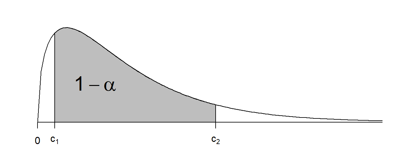
Figure 3.1: Probability density function of the chi-squared distribution
The standard approach is to choose \(c_{1}\) and \(c_{2}\) so that \[\begin{eqnarray*} P \left( \frac{(n-1)S^{2}}{\sigma^{2}} < c_{1} \right) &=& \alpha/2 \mbox{, and} \\ P \left(\frac{(n-1)S^{2}}{\sigma^{2}} > c_{2} \right) &=& \alpha/2 \end{eqnarray*}\] Thus, we choose \[\begin{eqnarray*} c_{1} \ = \ \chi^{2}_{n-1, \alpha/2}, & \ & c_{2} \ = \ \chi^{2}_{n-1, 1-\alpha/2} \end{eqnarray*}\] where \(P(V \leq \chi^{2}_{\nu, p})=p\) for \(V \sim \chi^{2}_{\nu}.\) Thus a \(100\times(1 - \alpha)\%\) confidence interval for \(\sigma^{2}\) is \[\begin{eqnarray*} \left(\frac{(n-1)s^{2}}{\chi^{2}_{n-1, 1-\alpha/2}}, \frac{(n-1)s^{2}}{\chi^{2}_{n-1, \alpha/2}} \right). \end{eqnarray*}\]
Remark: How do we find the quantiles and probabilities of the chi-squared distribution?
If \(V \sim \chi^{2}_{\nu}\) let \(P(V \leq \chi^{2}_{\nu, p})=p\).
In the University Formula Book, Section B4 tabulates the percentage points of the \(\chi^{2}\)-distribution. Note that it gives upper-tail values and so you will need to take care that you find the correct value. In the table, the rows correspond to the degrees of freedom, \(\nu\) and the columns the upper-tail probability. Thus, if you want a lower tail probability of \(p\) this corresponds to an upper tail probability of \(1-p\). For example, \(P(\chi^{2}_{8} \leq 2.180) = 0.025\) since (using the table) \(P(\chi^{2}_{8} > 2.180) = 0.975\). Similarly, \(P(\chi^{2}_{8} \leq 17.535) = 0.975\) since (using the table) \(P(\chi^{2}_{8} > 17.535) = 0.025\).
In
R, for a given \(\nu\) and \(p\), \(\chi^{2}_{\nu, p}\) may be found using the commandqchisq(\(p,\nu\)). For a given \(\chi^{2}_{\nu, p}\), \(p\) may be found using the commandpchisq(\(\chi^{2}_{\nu, p}, \nu\)).# Let V be a chi-squared distribution with 8 degrees of freedom qchisq(0.025, 8) # finds v such that P(V <= v) = 0.025## [1] 2.179731## [1] 0.02500977
- To directly compute an upper tail probability, or corresponding quantile, in
Ryou need to change the default inpchisqorqchisqto calculate the upper tail.# Let Y be a chi-squared distribution with 8 degrees of freedom qchisq(0.025, 8, lower.tail=F) # finds y such that P(Y > y) = 0.025## [1] 17.53455## [1] 0.04954038
Example 3.3 (Confidence interval for variance of BMI in NHANES) Recall the NHANES BMI data from Example 1.7. BMI data are available on \(n= 1638\) observations. The sample variance was \(s^{2}= 46.51\). Assuming the population distribution of BMI is normal, and using the function
qchisqin R to find the required quantiles of the chi-squared distribution, we can construct a 95% confidence interval for the population variance of BMI as \[\begin{eqnarray*} \left(\frac{1637 \times 46.51}{1751.029}, \frac{1637 \times 46.51}{1526.759}\right) & = & (43.482, 49.869). \end{eqnarray*}\] This confidence interval was constructed assuming the population distribution of BMI values is normal. Given Figure 1.1 we should therefore be cautious about our results given that the normality assumption is somewhat tenable.
3.2.2 Confidence interval for the mean with unknown variance
In Example 3.2, we constructed a \(100 \times (1-\alpha)\)% confidence interval for a normal mean \(\mu\) when the variance was assumed to be known. This result is not practically very useful because it would be rare that we would know the true value of \(\sigma^{2}.\) We now consider the more realistic case where both \(\mu\) and \(\sigma^{2}\) are unknown. To do this, we introduce a new distribution, the t-distribution.
Definition 3.4 (t-distribution) If \(Z \sim N(0,1),\) \(U \sim \chi^{2}_{\nu},\) and \(Z\) and \(U\) are independent, then the distribution of \(\frac{Z}{\sqrt{U/\nu}}\) is called the t-distribution with \(\nu\) degrees of freedom.
As shown in Figure 3.2, the t-distribution is symmetric around zero, and looks similar to the normal. It differs from the normal in that it has fatter tails, meaning there is more probability on values far away from the center than with the normal distribution. As the degrees of freedom increase, the t-distribution density converges to the standard normal density.
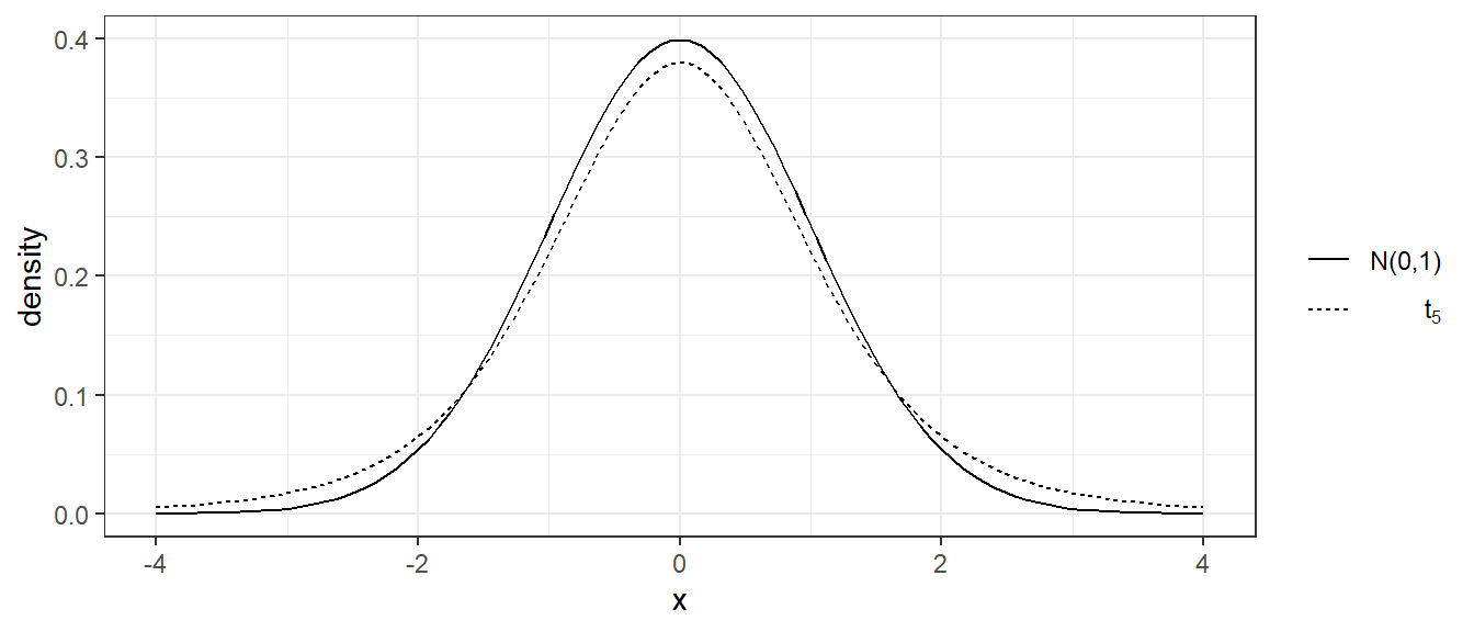
Figure 3.2: Standard normal and t-distribution (5 d.f.) density functions
Recall that \(\frac{\overline{X}-\mu}{\sigma/\sqrt{n}} \sim N(0,1)\) and \(\frac{(n-1)S^{2}}{\sigma^{2}} \sim \chi^{2}_{n-1}.\) Now we note that \[\begin{eqnarray*} \frac{\frac{\overline{X}-\mu}{\tfrac{\sigma}{\sqrt{n}}}} {\sqrt{\frac{S^{2}}{\sigma^{2}}}} = \frac{\overline{X}-\mu}{S/\sqrt{n}}. \end{eqnarray*}\] Lastly, we recall that \(\overline{X}\) and \(S^{2}\) are independent. We have thus shown that \[\begin{eqnarray*} \frac{\overline{X}-\mu}{S/\sqrt{n}} \sim t_{n-1}. \end{eqnarray*}\] This quantity is thus is pivot for \(\mu\), enabling us to form a confidence interval. Proceeding analogously to the case where \(\sigma^{2}\) was known, suppose we have chosen constants \(c_{1}\) and \(c_{2}\) such that \[\begin{eqnarray*} P(c_{1} < t_{n-1} < c_{2}) = 1-\alpha. \end{eqnarray*}\] Then we have that \[\begin{eqnarray*} P\left( c_{1} < \frac{\overline{X}-\mu}{S/\sqrt{n}} < c_{2} \right) = 1-\alpha \end{eqnarray*}\] and as before re-arranging we obtain \[\begin{eqnarray*} P\left(\overline{X}-c_{2} \frac{S}{\sqrt{n}} < \mu < \overline{X}-c_{1}\frac{S}{\sqrt{n}} \right) = 1-\alpha, \end{eqnarray*}\] thus allowing us to form a \(100 \times (1-\alpha)\)% confidence interval for \(\mu.\) If we choose to construct a symmetric interval, we can choose \(c_{1}=-c_{2}.\) If \(t_{\nu}\) is a \(t\)-distribution with \(\nu\) degrees of freedom, let \(t_{\nu,p}\) be such that \(P(t_{\nu} \leq t_{\nu,p})=p\). We choose \(c_{2}=t_{n-1,1-\alpha/2}\) so that our \(100 \times (1-\alpha)\)% confidence interval for \(\mu\) is given by \[\begin{equation} \left(\overline{X}-t_{n-1,1-\alpha/2} \frac{S}{\sqrt{n}}, \overline{X}+t_{n-1,1-\alpha/2} \frac{S}{\sqrt{n}} \right) \tag{3.2} \end{equation}\] or equivalently \(\overline{X}\pm t_{n-1,1-\alpha/2} S/\sqrt{n}\).
Remark: How do we find the quantiles and probabilities of the t-distribution?
If \(t_{\nu}\) is a \(t\)-distribution with \(\nu\) degrees of freedom, let \(P(t_{\nu} \leq t_{\nu,p})=p\).
In the University Formula Book, Section B3 tabulates the percentage points of the \(t\)-distribution. Note that it gives upper-tail values and so you will need to take care that you find the correct value. In the table, the rows correspond to the degrees of freedom and the columns the upper-tail probability. Thus, if you want a lower tail probability of \(p\) this corresponds to an upper tail probability of \(1-p\). For example, \(P(t_{8} \leq 2.896) = 0.99\) since (using the table) \(P(t_{8} > 2.896) = 0.01\).
In
R, for a given \(p\), \(t_{\nu, p}\) may be found using the commandqt(\(p, \nu\)). For a given \(t_{\nu, p}\), \(p\) may be found using the commandpt(\(t_{\nu, p}, \nu\))# Let T be a t-distribution with 8 degrees of freedom qt(0.99, 8) # finds t such that P(T <= t) = 0.99## [1] 2.896459## [1] 0.989993
- To directly compute an upper tail probability, or corresponding quantile, in
Ryou need to change the default inptorqtto calculate the upper tail.# Let T be a t-distribution with 8 degrees of freedom qt(0.01, 8, lower.tail=F) # finds t such that P(T > t) = 0.01## [1] 2.896459## [1] 0.01000705
Example 3.4 (Confidence interval for mean BMI in NHANES) In Example 2.8, we estimated the population mean BMI from the NHANES data by its sample mean \(\hat{\mu}=\overline{x}=\) 27.911. This was based on \(n=1638\) observations. The sample standard deviation was \(s= 6.82\).
The confidence interval limits for a 95% confidence interval for the mean are given by \[\begin{eqnarray*} \left(27.911-t_{1637, 0.975}\frac{6.82}{\sqrt{1638}}, 27.911+t_{1637, 0.975}\frac{6.82}{\sqrt{1638}}\right). \end{eqnarray*}\] We calculate \(t_{1637, 0.975}\) in
Rusingqt(p = 0.975, df = 1637). Then the above expression evaluates to \[\begin{eqnarray*} (27.581, 28.242) \end{eqnarray*}\] Again, given Figure 1.1 which suggests the distribution of BMI values is not normal, we should be concerned about whether the normality assumption made in the construction of this confidence interval for the mean is reasonable.
3.3 Confidence intervals for the exponential distribution
Consider an i.i.d. sample from the exponential distribution with rate parameter \(\lambda.\) We showed in Example 2.3 that the MLE for \(\lambda\) is \(\hat{\lambda}=1/\overline{x}.\) We now consider how to form a confidence interval for \(\lambda.\) We first note that the exponential is a special case of the Gamma distribution. Specifically, a Gamma distribution with shape 1 and rate \(\lambda,\) which we will denote by \(Ga(\lambda,1),\) is exponentially distributed with rate \(\lambda.\) We will need to use the following result from probability theory:
Theorem 3.2 Let \(X_{1}, \ldots,X_{n}\) be i.i.d. from \(Ga(\lambda,k)\) with shape parameter \(k>0.\) Then for \(c>0,\) \[\begin{eqnarray*} c \sum^{n}_{i=1} X_{i} \sim Ga(\lambda/c,nk) \end{eqnarray*}\]
Proof: See your Probability & Statistics 1B notes for the proof. \(\Box\)
It follows from Theorem 3.2 that if \(X_{1}, \ldots,X_{n}\) are i.i.d. \(Exp(\lambda)=Ga(\lambda,1)\) \[\begin{eqnarray*} \sum^{n}_{i=1} X_{i} \sim Ga(\lambda,n) \quad \text{ and so } \quad \lambda \sum^{n}_{i=1} X_{i} \sim Ga(1,n) \end{eqnarray*}\] and thus we have a pivot for \(\lambda.\) In particular \[\begin{eqnarray*} \alpha/2 = P\left(\lambda n \overline{X} < Ga_{1,n,\alpha/2} \right) = P\left(\lambda < \frac{Ga_{1,n,\alpha/2}}{n \overline{X}}\right) \end{eqnarray*}\] where \(Ga_{1,n,\alpha/2}\) denotes the \(\alpha/2\) percentile of the Gamma distribution with shape \(n\) and rate 1, and \[\begin{eqnarray*} \alpha/2 = P(\lambda n \overline{X} > Ga_{1,n,1-\alpha/2}) = P\left(\lambda > \frac{Ga_{1,n,1-\alpha/2}}{n \overline{X}}\right) \\ \end{eqnarray*}\] so we can construct an equitailed \(100\times(1-\alpha)\)% confidence interval for \(\lambda\) as \[\begin{eqnarray*} \left(\frac{Ga_{1,n,\alpha/2}}{n \overline{X}}, \frac{Ga_{1,n,1-\alpha/2}}{n \overline{X}}\right). \end{eqnarray*}\]
3.4 Robustness to model misspecification
The confidence intervals we have just constructed relied on parametric assumptions that the individual observations (in the population) are normally or exponentially distributed. Note that this is an assumption about the data generating mechanism or the infinite population from which we have sampled – it is not a property of the sample of observed data. Thus although there exist various methods for checking modelling assumptions, we can never prove from the observed data that a particular modelling assumption is true. It is therefore extremely useful if we can derive methods which are valid (usually approximately) under weaker modelling assumptions.
To make progress in this direction, we recall the Central Limit Theorem (CLT) from Probability & Statistics 1B.
Theorem 3.3 (Central Limit Theorem (CLT)) Let \(X_{1}, \ldots,X_{n}\) be i.i.d. from a distribution with finite mean \(\mu\) and finite variance \(\sigma^{2}.\) Let \(\overline{X}_{n}=n^{-1}\sum^{n}_{i=1} X_{i}.\) Then as \(n \rightarrow \infty\) \[\begin{eqnarray*} \sqrt{n}(\overline{X}_{n} - \mu) / \sigma \approx N(0, 1) \end{eqnarray*}\]
Proof: A sketch proof can be found in Appendix A.5 of Lehmann, and references therein. \(\Box\)
The convergence being asserted by the CLT is known as convergence in distribution, or convergence in law:
Definition 3.5 (Convergence in law) Let \((A_{n})_{n \in \mathbb{N}}\) be a sequence of random variables with corresponding cumulative distribution functions \(F_{n}(\cdot),\) and let \(A\) have cumulative distribution function \(F(\cdot).\) Suppose that \(F_{n}(a) \rightarrow F(a)\) at all continuity points \(a\) of \(F(\cdot).\) Then we say that \(A_{n}\) converges in distribution or law to \(A,\) which we write as \[\begin{eqnarray*} A_{n} \xrightarrow{L} A \end{eqnarray*}\]
If the distribution of \(A\) is a commonly-used distribution, e.g. \(N(0,1),\) it is convention (although notationally not really correct) to write this as \(A_{n} \xrightarrow{L} N(0,1).\) Now we can more precisely restate the final line in the CLT as \[\begin{eqnarray*} \sqrt{n}(\overline{X}_{n} - \mu) / \sigma \xrightarrow{L} N(0, 1). \end{eqnarray*}\]
If \(\sigma^{2}\) were known, the CLT enables us to use the same confidence interval that we constructed in Example 3.2 for the mean of a normal distribution and apply it to situations where the normality assumption may not hold, i.e. for large \(n\) \[\begin{eqnarray*} P \left( \overline{X} - z_{1-\alpha/2} \frac{\sigma}{\sqrt{n}} < \mu < \overline{X} + z_{1-\alpha/2} \frac{\sigma}{\sqrt{n}} \right) \approx 1-\alpha \end{eqnarray*}\] We will consider how good the approximation is shortly.
The usefulness of this result is limited by the fact that in practice the variance \(\sigma^{2}\) is typically not known. We know that we can estimate \(\sigma^{2}\) unbiasedly by \(S^{2}.\) One might therefore be tempted to use the preceding confidence interval, replacing the unknown \(\sigma\) by the estimate \(S.\) The question is, can this be justified? As long as \(S\) is consistent, the answer turns out to be ‘yes’, due to Slutsky’s Theorem:
Theorem 3.4 (Slutsky's Theorem) If \(Y_{n} \xrightarrow{L} Y,\) \(A_{n} \xrightarrow{P} a,\) \(B_{n} \xrightarrow{P} b,\) then \[\begin{eqnarray*} A_{n} + B_{n} Y_{n} \xrightarrow{L} a + b Y \end{eqnarray*}\]
Proof: Omitted. See Theorem A.14.9 of Bickel and Doksum. \(\Box\)
We can now use Slutsky’s Theorem to justify replacing the unknown \(\sigma\) by \(\hat \sigma\) in the Central Limit Theorem:
Proposition 3.1 Let \(X_{1}, \ldots,X_{n}\) be i.i.d. from a distribution with finite mean \(\mu\) and finite variance \(\sigma^{2}.\) Let \(\hat{\sigma}\) be a consistent estimator of \(\sigma.\) Then \[\begin{eqnarray*} \frac{(\overline{X}_{n}-\mu)}{\hat{\sigma}/\sqrt{n}} \xrightarrow{L} N(0,1). \end{eqnarray*}\]
Sketch proof: Apply the CLT to \(\left(\overline{X}_{n}-\mu\right)/(\sigma/\sqrt{n})\) and then multiply by \(\sigma/\hat{\sigma}\) and invoke Slutsky. \(\Box\)
And finally we can justify replacing \(\sigma\) by \(S\) in the z-interval, assuming \(S\) is a consistent estimator for \(\sigma\) (see conditions in Proposition 2.2):
Proposition 3.2 Let \(X_{1}, \ldots,X_{n}\) be i.i.d. from a distribution with mean \(\mu\) and finite variance \(\sigma^{2}.\) Assume \(S\) is a consistent estimator for \(\sigma\). Then the interval \[\begin{equation} \left( \overline{X} - z_{1-\alpha/2} \frac{S}{\sqrt{n}} , \overline{X} + z_{1-\alpha/2} \frac{S}{\sqrt{n}} \right) \tag{3.3} \end{equation}\] is asymptotically an \(100 \times (1-\alpha)\)% confidence interval for \(\mu.\)
Sketch Proof: Applying proposition 3.1 and the consistency of \(S,\) \(\frac{\sqrt{n}(\overline{X}_{n}-\mu)}{S}\) is (approximately) a pivot for \(\mu,\) so \[\begin{eqnarray*} P \left( \overline{X}_n - z_{1-\alpha/2} \frac{S}{\sqrt{n}} < \mu < \overline{X}_n + z_{1-\alpha/2} \frac{S}{\sqrt{n}} \right) = 1-\alpha \end{eqnarray*}\] as \(n \rightarrow \infty.\) \(\Box\)
For full proofs of these two propositions, see Chapter 6.
Definition 3.6 (Coverage probability) The coverage probability is the probability that a procedure for constructing confidence intervals will produce an interval containing, or covering, the true value.
The coverage probability is a property of the procedure itself rather than of a particular confidence interval produced based on a sample of data. There are no guarantees that confidence intervals constructed based on the preceding asymptotic derivations will have the nominal \(100\times(1-\alpha)\)% coverage for finite \(n\).
Consider the confidence interval in Equation (3.3). The first thing to note is that if it were actually the case that \(X_{1}, \ldots,X_{n}\) were normally distributed and we estimate \(\sigma\) by \(S,\) the t-interval \[\begin{eqnarray*} \left(\overline{X}-t_{n-1,1-\alpha/2} \frac{S}{\sqrt{n}}, \overline{X}+t_{n-1,1-\alpha/2} \frac{S}{\sqrt{n}} \right) \end{eqnarray*}\] has coverage \(100 \times (1-\alpha)\)%. Since the t-distribution has fatter tails than the normal, \(t_{n-1,1-\alpha/2} > z_{1-\alpha/2},\) we can immediately deduce that were the population really normally distributed, the z-interval \[\begin{equation*} \left( \overline{X} - z_{1-\alpha/2} \frac{S}{\sqrt{n}} , \overline{X} + z_{1-\alpha/2} \frac{S}{\sqrt{n}} \right) \end{equation*}\] must have coverage somewhat less than \(100 \times (1-\alpha)\)% for finite \(n.\) One option is therefore to use the t-interval rather than the z-interval, because we know that in the case of normally distributed data this is the right thing to do, and asymptotically they are identical. When the normality assumption for \(X_{1}, \ldots,X_{n}\) does not hold, how good the approximation is will depend on how far from normality the true distribution is and the sample size \(n.\)
Example 3.5 Recall that Figure 1.1 for the NHANES BMI data suggests an assumption of normality for the population distribution of BMI may not be reasonable, raising doubts about the validity of the confidence interval we calculated in Example 3.4. However, given the relatively large sample size of \(n= 1638,\) the preceding results give us some reassurance that the apparent non-normality of the distibution ought not to overly concern us.
To investigate what sample size \(n\) might be sufficient for the sample mean BMI based on \(n\) observations \(\overline{X}_{n}\) to be approximately normally distributed, we perform a small simulation study. Figure 3.3 shows four histograms. For four different values of \(n,\) they show the distribution of the \(\overline{X}_{n}\) based on 10,000 samples taken from the original data, i.e. the \(n=1638\) observed BMI values. Taking new samples from the original sample in this way is not the same thing as taking samples from the population, but if the original sample is not too small, it turns out that resampling the original sample will give us similar results to taking repeated samples from the population (this idea is the basis of the important method called bootstrapping).
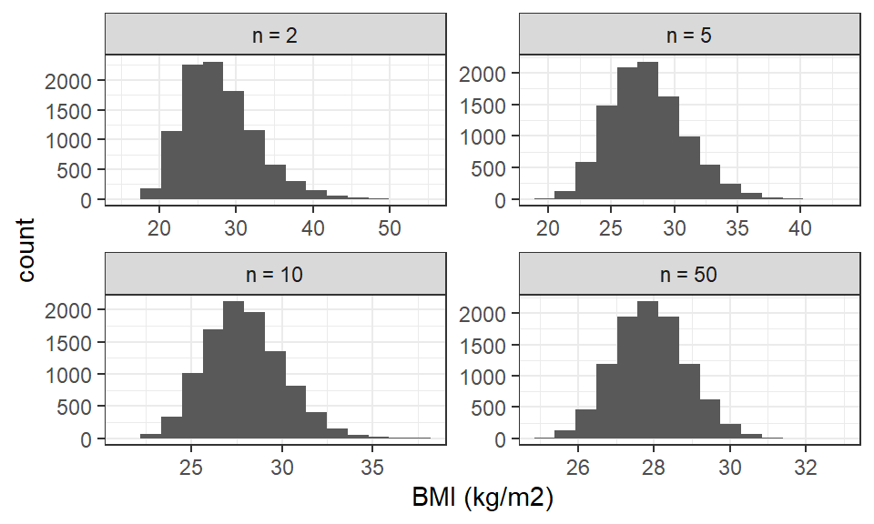
Figure 3.3: Distribution of sample mean of BMI for increasing sample sizes
The figure shows that with \(n=2,\) \(\overline{X}_{n}\) still has a skewed, non-normal distribution. As \(n\) is increased, we see that the distribution of \(\overline{X}_{n}\) begins to look much closer to a normal. Visually, it would appear that \(n=50\) would be sufficient here for \(\overline{X}_{n}\) to be approximately normal. This is reassuring in regards the validity of the confidence interval calculated in Example 3.4.
The confidence interval we have used for the mean uses \(S\) to estimate \(\sigma,\) but the proof of Proposition 3.2 only relied on \(S\) in so far as it was a consistent estimator for \(\sigma.\) It is thus easy to generalise this result by allowing any consistent estimator of \(\sigma\) to be used:
Example 3.6 Let \(X_1,\ldots,X_n\) be i.i.d. Bernoulli(\(p\)). Recall that for this model, \(E(X)=p\) and \(\text{Var}(X)=p(1-p).\) We showed in Example 2.4 that the MLE of \(p\) is \(\hat{p}=\overline{X},\) and (from a problems class) that \(\hat{p}(1-\hat{p})\) is consistent for \(\text{Var}(X)=p(1-p).\) By the Continuous Mapping Theorem (Theorem 2.4) we then have that \[\begin{eqnarray*} \sqrt{\hat{p}(1-\hat{p})} \xrightarrow{P} \sqrt{\text{Var}(X)} \end{eqnarray*}\] Thus by Proposition 3.1 we have that \[\begin{eqnarray*} \frac{\overline{X}_{n}-p}{\sqrt{\frac{\overline{X}_{n}(1-\overline{X}_{n})}{n}}} \xrightarrow{L} N(0,1) \end{eqnarray*}\] For finite \(n,\) we can use this result to say that \[\begin{eqnarray*} P\left(-z_{1-\alpha/2} < \frac{\overline{X}_{n}-p}{\sqrt{\frac{\overline{X}_{n}(1-\overline{X}_{n})}{n}}} < z_{1-\alpha/2}\right) \approx 1-\alpha \end{eqnarray*}\] so that \[\begin{equation} P\left(\overline{X}_{n}-z_{1-\alpha/2}\sqrt{\frac{\overline{X}_{n}(1-\overline{X}_{n})}{n}} < p <\overline{X}_{n} + z_{1-\alpha/2} \sqrt{\frac{\overline{X}_{n}(1-\overline{X}_{n})}{n}} \right) \approx 1-\alpha \tag{3.4} \end{equation}\]
An alternative to estimating \(\text{Var}(X)\) by \(\hat{p}(1-\hat{p})\) would be to estimate it by \(S^2.\) For large \(n\) they will be very close.
Figure 3.4 shows the empirical coverage of this interval for \(\alpha=0.05\) and for different true values of \(p.\)
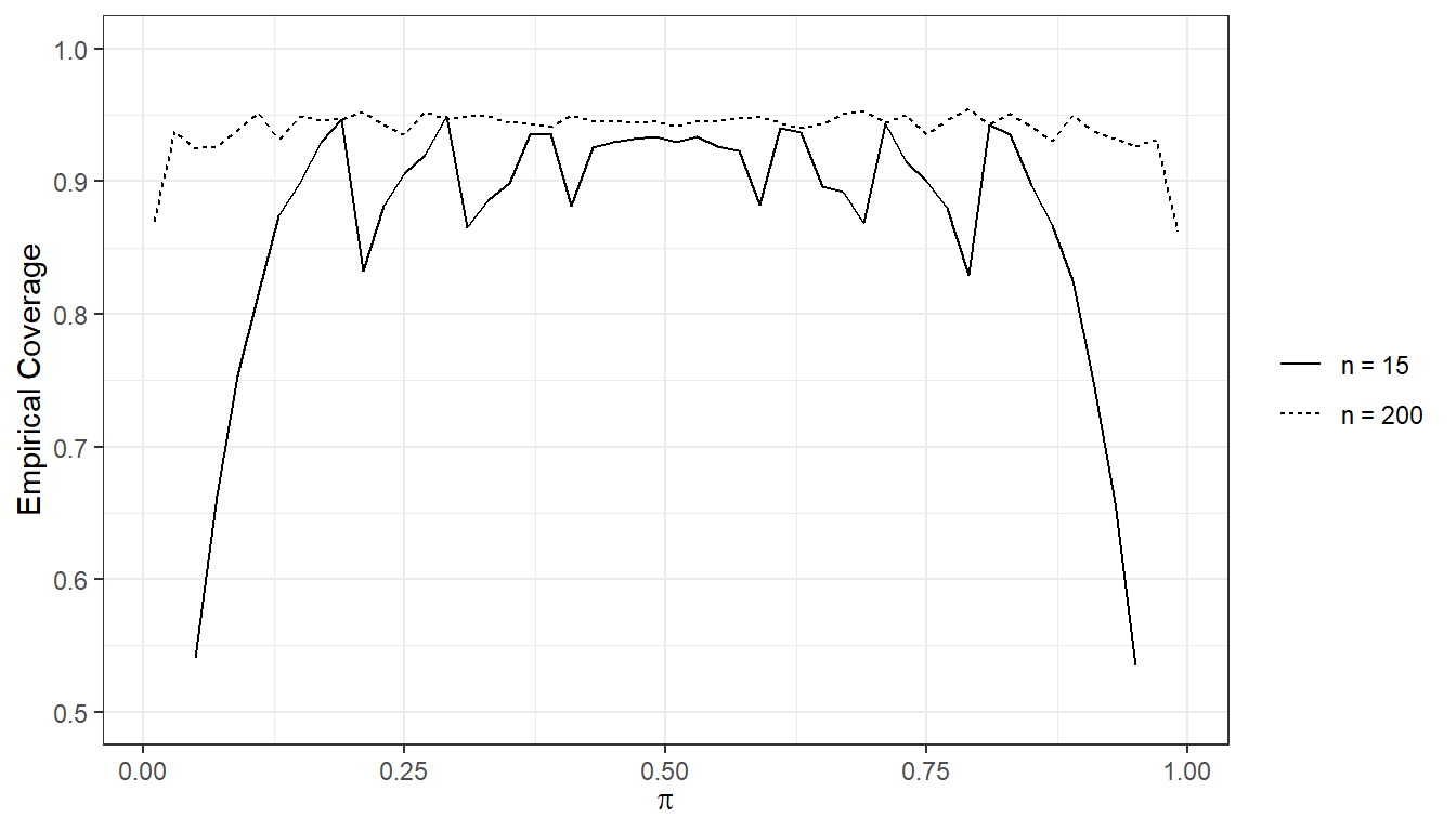
Figure 3.4: Simulated empirical coverage of nominal 95\(\%\) confidence intervals for \(p\)
For each combination of \(p,\) and \(n=15\) or \(n=200,\) the coverage is estimated by
- repeatedly simulating \(X_1,\ldots,X_n\) as i.i.d. Bernoulli(\(p\)) a large number (say 10,000) times
- computing a confidence interval for \(p\) using Equation (3.4) for each simulation
- calculating the proportion of these 10,000 repetitions which contain the true value of \(p\) (treating the intervals as closed intervals).
We can then compare this empirical coverage to the nominal coverage of \(100(1-\alpha)\%.\) It is clear that the empirical coverage improves (is closer to the nominal level) with increasing \(n,\) and it is also better when \(p\) is closer to 0.5.
Example 3.7 Recall from Example 1.8 the data on alcohol consumption from NHANES. For this variable \(n=1,104\) responded to the question, and of these, 846 (76.6%) answered that they drank more than one alcoholic drink on average on days that they did drink alcohol. We can use the i.i.d. Bernoulli model here, with \(p\) representing the proportion of the population that would answer that they drink more than one alcoholic drink on average on days they drink. The MLE is \(\hat{p}=846/1104.\) We can construct an asymptotic 95% confidence interval for \(p\) using the limits in the inequality in Equation (3.4). This gives \[\begin{eqnarray*} \left(\frac{846}{1104}-1.96\sqrt{\frac{\frac{846}{1104}(1-\frac{846}{1104})}{1104}}, \frac{846}{1104} + 1.96 \sqrt{\frac{\frac{846}{1104}(1-\frac{846}{1104})}{1104}} \right), \end{eqnarray*}\]
which evaluates to (0.7413413,0.7912674).
3.5 Summary of confidence intervals
This section contains a summary of the key confidence intervals we have covered in this chapter.
3.5.1 Normal model
\(X_{1}, \ldots,X_{n}\) i.i.d. \(N(\mu,\sigma^{2}).\)
If \(\sigma\) is known, a \(100\times (1-\alpha)\)% confidence interval for \(\mu\) is \[\begin{equation*} \left( \overline{X} - z_{1-\alpha/2} \frac{\sigma}{\sqrt{n}} , \overline{X} + z_{1-\alpha/2} \frac{\sigma}{\sqrt{n}} \right) \end{equation*}\] where if \(Z \sim N(0, 1)\), \(P(Z \leq z_{1-\alpha/2}) = 1 - \alpha/2\).
If \(\sigma\) is unknown and estimated by \(S,\) a \(100\times (1-\alpha)\)% confidence interval for \(\mu\) is \[\begin{equation*} \left(\overline{X}-t_{n-1,1-\alpha/2} \frac{S}{\sqrt{n}}, \overline{X}+t_{n-1,1-\alpha/2} \frac{S}{\sqrt{n}} \right) \end{equation*}\] where if \(t_{n-1}\) is the \(t\)-distribution with \(n-1\) degrees of freedom, \(P(t_{n-1} \leq t_{n-1,1-\alpha/2}) = 1 - \alpha/2\).
Again with \(\sigma\) and \(\mu\) unknown, a \(100\times (1-\alpha)\)% confidence interval for \(\sigma^{2}\) is \[\begin{eqnarray*} \left(\frac{(n-1)S^{2}}{\chi^{2}_{n-1, 1-\alpha/2}}, \frac{(n-1)S^{2}}{\chi^{2}_{n-1, \alpha/2}} \right) \end{eqnarray*}\] where if \(\chi^{2}_{n-1}\) is the chi-squared distribution with \(n-1\) degrees of freedom, \(P(\chi^{2}_{n-1} \leq \chi^{2}_{n-1, \alpha/2}) = \alpha/2\) and \(P(\chi^{2}_{n-1} \leq \chi^{2}_{n-1, 1-\alpha/2}) = 1 - \alpha/2\).
3.5.2 Robustness of confidence intervals for the mean
If the normality assumption is removed, provided the mean and variance of \(X\) are finite, the z and t intervals above have the correct coverage asymptotically, and for finite \(n\) will have approximately the correct coverage.
3.5.3 Asymptotic confidence intervals for means
Let \(f(x|\theta)\) be some parametric model with finite mean \(\mu\) and finite variance \(\sigma^{2},\) each of which are functions of the model parameter(s) \(\theta.\) Let \(\hat{\sigma}\) be a consistent estimator of \(\sigma.\) Then asymptotically, the following confidence interval has coverage \(100\times (1-\alpha)\)% for \(\mu:\) \[\begin{eqnarray*} \left( \overline{X} - z_{1-\alpha/2} \frac{\hat{\sigma}}{\sqrt{n}} , \overline{X} + z_{1-\alpha/2} \frac{\hat{\sigma}}{\sqrt{n}} \right) \end{eqnarray*}\]