Chapter 4 Hypothesis testing

4.1 Introduction to statistical hypothesis testing

In this chapter we introduce hypothesis testing for parameters in a statistical model. Suppose we have a model parameter \(\theta \in \Theta.\) A hypothesis is a statement that the true value of \(\theta\) belongs in some subset of the parameter space \(\Theta.\) The null hypothesis, denoted \(H_{0},\) specifies one such subset. The alternative hypothesis, denoted \(H_{1}\), specifies another subset. In the Neyman-Pearson framework of hypothesis testing, we use the data to construct a test that will either result in our accepting the null hypothesis \(H_{0}\) or rejecting this in favour of the alternative hypothesis \(H_{1}.\)

Example 4.1 (Manufacturing defects) Suppose a machine in a factory is known to produce defective items 20% of the time. The machine is sent for repairs and then re-introduced to the production line. The factory managers want to know if the proportion of defective products being produced by the machine has been reduced after the repairs. Letting \(p\) denote the probability of an item being defective, we are interested in testing \(H_{0}: p=0.2\) versus \(H_{1}: p < 0.2.\)

Example 4.2 (Two arm clinical trial) In a two arm randomised clinical trial (c.f., Example 1.9) the true population mean outcome under control treatment is \(\mu_{0}\) and is \(\mu_{1}\) on the new treatment. The company developing the new treatment seeks a license to sell the new drug and needs to demonstrate to the regulatory agencies evidence in support of the hypothesis that \(\mu_{1}>\mu_{0}.\) Thus the null hypothesis might be taken to be \(H_{0} : \mu_{1} = \mu_{0}\) (the mean of the outcome is the same under treatment and control) and the alternative hypothesis \(H_{1}: \mu_{1} > \mu_{0}\) (the mean of the outcome is greater in the treatment arm).

To construct a hypothesis test we choose a test statistic: a statistic \(T(X_{1}, \ldots,X_{n})\) which is a function of the observed data. The basic idea is that the test statistic is measuring the relative compatibility of the observed data with the two hypotheses. Next we define the critical region.

Definition 4.1 (Critical Region) Let \(\mathcal T\) denote the sample space of values of the test statistic \(T.\) The region \(C \subseteq \mathcal T\) for which \(H_{0}\) is rejected in favour of \(H_{1}\) is termed the critical (or rejection) region while the region \(\mathcal T \setminus C,\) where we accept \(H_{0},\) is called the acceptance region. The critical and acceptance regions can also equivalently be defined in terms of the subset of the sample space of the data for which we reject or accept \(H_{0}.\)

The substantive question of interest typically dictates the specification of the null and alternative hypotheses. The question is thus how we should choose the test statistic and the critical region.

4.2 Tests for simple hypotheses

If a hypothesis completely specifies the probability distribution of \(X\) then it is said to be a simple hypothesis. If the hypothesis is not simple then it is said to be composite. In this section we will consider the case where \(H_{0}\) and \(H_{1}\) are both simple hypotheses. This means that \(H_{0}\) specifies that the data are distributed according to a specific distribution, and similarly for \(H_{1}.\) The developments for the case where both \(H_{0}\) and \(H_{1}\) are simple are easier than the case where one or both of the hypotheses are composite, which we will consider in the next section.

4.2.1 Evaluating a test

In the paradigm of hypothesis testing developed by Neyman and Pearson, we reject or accept \(H_{0}\) based on whether the value of the test statistic falls within the critical region. Unless we have an infinite amount of data, there is a non-zero probability that we may reject \(H_{0}\) when it is in fact true or accept \(H_{0}\) when it is actually false. Table 4.1 summarises the possible outcomes.

Table 4.1: Possible outcomes and types of error in a hypothesis test.

	ACCEPT \(H_{0}\)	REJECT \(H_{0}\)
\(H_{0}\) TRUE	CORRECT	ERROR (Type I)
\(H_{0}\) FALSE	ERROR (Type II)	CORRECT

Definition 4.2 (Type I and Type II errors) A Type I error occurs when \(H_{0}\) is rejected when it is true. The probability of such an error is denoted by \(\alpha\) so that \[\begin{eqnarray*} \alpha \ = \ P(\mbox{Type I error}) \ = \ P(\mbox{Reject $H_{0}$} \, | \, \mbox{$H_{0}$ true}). \end{eqnarray*}\] A Type II error occurs when \(H_{0}\) is accepted when it is false. The probability of such an error is denoted by \(\beta\) so that \[\begin{eqnarray*} \beta \ = \ P(\mbox{Type II error}) \ = \ P(\mbox{Accept $H_{0}$} \, | \, \mbox{$H_{0}$ false}). \end{eqnarray*}\]
The power is defined as \(1-\beta\) and is the probability we reject \(H_{0}\) when \(H_{0}\) is false.

Example 4.3 Suppose \(X_{1}, \ldots, X_{n}\) are i.i.d. normal with known variance \(\sigma^2\) and mean \(\mu\) either equal to \(\mu_{0}\) or \(\mu_{1}\) where \(\mu_1>\mu_0.\) Assume in this case that \(H_0:\,\mu=\mu_0\) and \(H_1:\,\mu=\mu_1\) and that the test statistic used is \(T=\overline{X}.\) Under \(H_{0},\) \(\overline{X} \sim N(\mu_{0}, \sigma^{2}/n)\) while under \(H_{1},\) \(\overline{X} \sim N(\mu_{1}, \sigma^{2}/n).\) A large observed value of \(\overline{x}\) may indicate that \(H_{1}\) rather than \(H_{0}\) is true. Intuitively, we may consider a critical region of the form \[\begin{eqnarray*} C & = & \{\overline{x} : \overline{x} \geq c\}. \end{eqnarray*}\] This critical region is shown in Figure 4.1

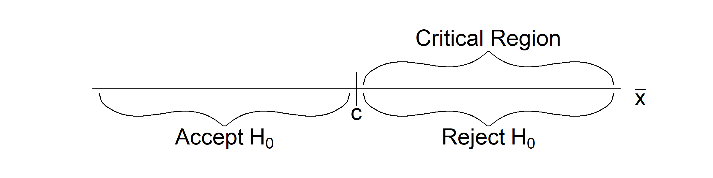
Figure 4.1: An illustration of the critical region \(C = \{\overline{x} : \overline{x} \geq c \}\)

There are a number of immediate questions. How should we pick the value of \(c,\) and how will its choice affect the probability of making Type I and Type II errors? We would like to make the probability of either of these errors as small as possible.

Figure 4.2 shows schematically how the choice of \(c\) can be expected to qualitatively alter these two probabilities.

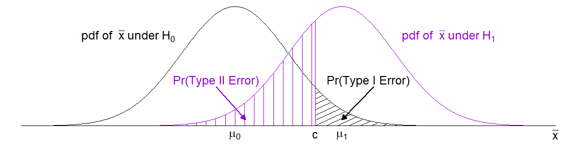
Figure 4.2: The errors resulting from the test with critical region \(C = \{\overline{x} : \overline{x} \geq c\}\) of \(H_{0}: \mu = \mu_{0}\) versus \(H_{1}: \mu = \mu_{1}\) where \(\mu_{1} > \mu_{0}.\)

It is clear from the figure that:

• If we INCREASE \(c\) then the probability of a Type I error DECREASES but the probability of a Type II error INCREASES.
• If we DECREASE \(c\) then the probability of a Type I error INCREASES but the probability of a Type II error DECREASES.

It turns out, in practice, that this is always the case: in order to decrease the probability of a Type I error, we must increase the probability of a Type II error and vice versa. We deal with this issue by fixing the probability of Type I error \(\alpha\) in advance.

Definition 4.3 (Significance level/Size of the test) When the probability of type I error \(\alpha\) is fixed in advance of observing the data then \(\alpha\) is known as the significance level of the test. In this context \(\alpha\) is also known as the size of the test.

We usually fix \(\alpha\) at some small value, say \(\alpha = 0.1, 0.05, 0.01, \ldots.\) Given a test statistic, fixing \(\alpha\) determines the critical region. It is important to note that by doing this we introduce some asymmetry to the setup: controlling the probability of a Type I error implies that it is the null hypothesis (rather than the alternative) that we want to ensure is not rejected too often when it is in fact true. In most cases the choice of \(\alpha\) level is arbitrary. The choice of \(\alpha=0.05\) has become essentially the world’s default \(\alpha\) level based on Sir Ronald Fisher’s suggestion of it being a potentially reasonable value, rather than a value that should be automatically and universally used.

Example 4.4 In Example 4.3 we considered a critical region of the form \[\begin{eqnarray*} C & = & \{\overline{x} : \overline{x} \geq c\}. \end{eqnarray*}\]
Now, \[\begin{eqnarray*} \alpha \ = \ P(\mbox{Type I error}) & = & P(\mbox{Reject $H_{0}$} \, | \, \mbox{$H_{0}$ true}) \\ & = & P\left(\overline{X} \geq c \, | \, \overline{X} \sim N(\mu_{0}, \sigma^{2}/n)\right) \\ & = & P\left(Z \geq \frac{c - \mu_{0}}{\sigma/\sqrt{n}}\right), \end{eqnarray*}\] where \(Z \sim N(0, 1).\) Suppose we choose \(\alpha = 0.05.\) We can then find the value of \(c\) which gives us \(\alpha=0.05\): \[\begin{eqnarray*} P\left(Z \geq \frac{c - \mu_{0}}{\sigma/\sqrt{n}}\right) & = & 0.05 \ \Rightarrow \\ \frac{c - \mu_{0}}{\sigma/\sqrt{n}} & = & 1.645 \ \Rightarrow \\ c & = & \mu_{0} + 1.645\frac{\sigma}{\sqrt{n}}. \end{eqnarray*}\] Notice that as \(n\) increases then \(c\) tends towards \(\mu_{0}.\) Also notice how as the (assumed known) standard deviation \(\sigma\) decreases, \(c\) also gets closer to \(\mu_{0}.\)

Once the significance level \(\alpha\) has been chosen, and hence the critical region, \(\beta\) and the power (\(1-\beta\)) are determined. It typically depends upon the sample size.

Example 4.5 Using the critical region given in Example 4.4 we find \[\begin{eqnarray*} \beta \ = \ P(\text{Type II error}) & = & P(\text{Accept } H_{0} \, | \, H_{1} \text{ true}) \\ & = & P\left(\overline{X} < c \, | \, \overline{X} \sim N(\mu_{1}, \sigma^{2}/n)\right) \\ & = & P\left(Z < \frac{c - \mu_{1}}{\sigma/\sqrt{n}}\right). \end{eqnarray*}\] The corresponding value of \(\beta\) is \[\begin{eqnarray*} \beta \ = \ P\left(Z < \frac{c - \mu_{1}}{\sigma/\sqrt{n}}\right) & = & P\left(Z < \frac{(\mu_{0} - \mu_{1}) + 1.645\sigma/\sqrt{n}}{\sigma/\sqrt{n}}\right) \\ & = & \Phi\left(1.645 - \frac{\sqrt{n}(\mu_{1} - \mu_{0})}{\sigma}\right) \end{eqnarray*}\] where \(P(Z < z) = \Phi(z).\) Note that as \(n\) increases then \(\beta\) decreases to zero. Thus, the power is tending to 1 as \(n \rightarrow \infty.\)

4.2.2 Constructing tests

In the example above we chose the test statistic (the sample mean) solely on the basis of our intuition that large values of the sample mean are supportive of \(H_{1}\) and not supportive of \(H_{0}\) being true. One general approach is to construct tests based on the relative values of the likelihood function at the parameter values specified by the two competing hypotheses. Thus suppose we have a realization of data \(\mathbf x=(x_{1}, \ldots,x_{n}).\) Then we can define the likelihood ratio as \[\begin{eqnarray*} \omega(\mathbf x; \theta_{0}, \theta_{1}) & = & \frac{L(\theta_0 \, | \,\mathbf x)}{L(\theta_1 \, | \,\mathbf x)} \end{eqnarray*}\] where \(L(\theta \, | \,\mathbf x)=f(\mathbf x \, | \,\theta)\) is the likelihood function given \(\mathbf x.\) In the case that the data are i.i.d. from \(f(x \, | \,\theta),\) this statistic is \[\begin{eqnarray*} \omega(\mathbf x; \theta_{0}, \theta_{1}) & = & \frac{\displaystyle \prod_{i=1}^n f(x_i \, | \, \theta_0)}{\displaystyle \prod_{i=1}^n f(x_i \, | \, \theta_1)} \end{eqnarray*}\] We can now consider constructing tests based on \(\omega(\mathbf x; \theta_{0}, \theta_{1}).\) Small values of \(\omega\) imply that the data are more likely under \(H_{1}\) than \(H_{0},\) and this is therefore evidence in favour of \(H_{1}\) being true. Conversely large values of \(\omega\) are consistent with \(H_{0}.\) Thus we might construct tests that reject \(H_{0}\) when \(\omega(\mathbf x; \theta_{0}, \theta_{1}) \leq k\) for a value \(k\) which ensures the test has size \(\alpha.\)

Example 4.6 Suppose that \(X_{1}, \ldots, X_{n}\) are i.i.d. \(N(\mu, \sigma^{2})\) random variables with \(\sigma^{2}\) known. We shall derive \(\omega(\mathbf x; \mu_{0}, \mu_{1})\) for testing \[\begin{eqnarray*} H_{0}: \mu = \mu_{0} & \mbox{ versus } & H_{1}: \mu = \mu_{1} \end{eqnarray*}\] where \(\mu_{1} > \mu_{0}.\) From Example 2.2 we have that

\[\begin{eqnarray} \omega(x_{1}, \ldots, x_{n}; \mu_{0}, \mu_{1}) & = & \frac{L(\mu_{0} \, | \, \mathbf x)}{L(\mu_{1} \, | \, \mathbf x)} \nonumber \\ & = &\frac{\exp\left\{-\frac{1}{2\sigma^{2}} \sum_{i=1}^{n}(x_{i} - \mu_{0})^{2}\right\}}{\exp\left\{-\frac{1}{2\sigma^{2}} \sum_{i=1}^{n}(x_{i} - \mu_{1})^{2}\right\}} \nonumber \\ & = & \exp\left\{\frac{1}{2\sigma^{2}}\left(\sum_{i=1}^{n}(x_{i} - \mu_{1})^{2} - \sum_{i=1}^{n}(x_{i} - \mu_{0})^{2}\right)\right\}. \tag{4.1} \end{eqnarray}\]

Now, \[\begin{eqnarray} \sum_{i=1}^{n}(x_{i} - \mu_{1})^{2} - \sum_{i=1}^{n}(x_{i} - \mu_{0})^{2} & = & \sum_{i=1}^{n}(x_{i}^{2} - 2\mu_{1}x_{i} + \mu_{1}^{2}) - \sum_{i=1}^{n}(x_{i}^{2} - 2\mu_{0}x_{i} + \mu_{0}^{2}) \nonumber \\ & = & -2\mu_{1}n\overline{x} + n\mu_{1}^{2} + 2\mu_{0}n\overline{x} - n\mu_{0}^{2} \nonumber \\ & = & n(\mu_{1}^{2} - \mu_{0}^{2}) - 2n\overline{x}(\mu_{1} - \mu_{0}). \tag{4.2} \end{eqnarray}\]

Substituting Equation (4.2) into (4.1) gives \[\begin{align*} \omega(x_{1}, \ldots, x_{n}; \mu_{0}, \mu_{1}) = \exp\left\{\frac{1}{2\sigma^{2}}\left(n(\mu_{1}^{2} - \mu_{0}^{2}) - 2n\overline{x}(\mu_{1} - \mu_{0})\right)\right\}. \end{align*}\] The critical region for the corresponding test of \(H_{0}: \mu = \mu_{0}\) versus \(H_{1}: \mu = \mu_{1}\) \((\mu_{1} > \mu_{0})\) is thus \[\begin{eqnarray} C & = & \left\{(x_{1}, \ldots, x_{n}): \exp\left\{\frac{1}{2\sigma^{2}}\left(n(\mu_{1}^{2} - \mu_{0}^{2}) - 2n\overline{x}(\mu_{1} - \mu_{0})\right)\right\} \leq k \right\} \nonumber \\ & = & \left\{(x_{1}, \ldots, x_{n}): n(\mu_{1}^{2} - \mu_{0}^{2}) - 2n\overline{x}(\mu_{1} - \mu_{0}) \leq 2\sigma^{2}\log k \right\} \nonumber \\ & = & \left\{(x_{1}, \ldots, x_{n}): - 2n\overline{x}(\mu_{1} - \mu_{0}) \leq 2\sigma^{2}\log k + n(\mu_{0}^{2} - \mu_{1}^{2})\right\} \nonumber \\ & = & \left\{(x_{1}, \ldots, x_{n}): \overline{x} \geq \frac{-\sigma^{2}}{n(\mu_{1} - \mu_{0})}\log k + \frac{(\mu_{0} + \mu_{1})}{2}\right\} \tag{4.3} \\ & = & \{(x_{1}, \ldots, x_{n}): \overline{x} \geq k^{*}\}. \tag{4.4} \end{eqnarray}\] Note that, in Equation (4.3), we have used the fact that \(\mu_{1} - \mu_{0} > 0\). The critical region given in Equation (4.4) is identical to our intuitive interval derived in Example 4.3. For the test to be of significance \(\alpha\) we choose (see Example 4.4) \[\begin{align*} k^{*} = \mu_{0} + z_{1-\alpha}\frac{\sigma}{\sqrt{n}}, \end{align*}\] where \(z_{1 - \alpha}\) is the \((1-\alpha)\)-quantile of the standard normal distribution (i.e. \(P(Z \leq z_{1 - \alpha}) = 1-\alpha\).)

Constructing tests of two simple hypotheses based \(\omega(\mathbf x; \theta_{0}, \theta_{1})\) is useful in that it gives us a general prescription for how to construct a test statistic for testing two simple hypotheses. A natural question however is whether such tests can be improved upon? Thus we ask can we find a different test statistic \(T^{*}\) and critical region which, for the same sample size \(n,\) has the same value of \(\alpha = P(\mbox{Type I error})\) but a smaller \(\beta = P(\mbox{Type II error})\)? Equivalently, can we find the test with the largest power?

Definition 4.4 (Most powerful test) Consider the test of the hypotheses \[\begin{eqnarray*} H_{0}: \theta = \theta_{0} & \mbox{ versus } & H_{1}: \theta = \theta_{1}\,. \end{eqnarray*}\] A test with statistic \(T^{*}\) and critical region \(C^*\) is the most powerful test of significance level \(\boldsymbol \alpha\) if and only if any other test with statistic \(T'\) and critical region \(C'\) and the same significance level \(\alpha,\) has smaller power. That is \[\begin{align*} \alpha & =P(T^{*} \in C^*\, | \,\theta=\theta_0)=P(T' \in C'\, | \,\theta=\theta_0)\\ 1-\beta & = P(T^{*} \in C^*\, | \, \theta=\theta_1)>P(T' \in C' \, | \, \theta=\theta_1) \end{align*}\]

It turns out that when testing two simple hypotheses, tests based on \(\omega(\mathbf x; \theta_{0}, \theta_{1})\) are indeed optimal.

Lemma 4.1 (The Neyman-Pearson Lemma) Let \(X_{1}, \ldots, X_{n}\) be i.i.d. with density/mass function \(f(x|\theta).\) Consider the test of hypotheses \[\begin{eqnarray*} H_{0}: \theta = \theta_{0} & \mbox{ versus } & H_{1}: \theta = \theta_{1}\,. \end{eqnarray*}\] Then the test with critical region of the form \(\{\mathbf x : \omega(\mathbf x; \theta_{0}, \theta_{1}) \leq k\}\) with \(k\) chosen so that the test has size \(\alpha\) is the most powerful test of significance level \(\alpha.\)

Proof: See Theorem 8.3.12 of Casella and Berger for details. \(\Box\)

Example 4.7 Let \(X_{1}, \ldots,X_{n}\) be i.i.d. Bernoulli with success probability \(p,\) so that the sum \(Y=\sum^{n}_{i=1} X_{i}\) is then binomially distributed \(\text{Bin}(n,p).\) Consider testing \(H_{0}:p=p_{0}\) versus \(H_{1}: p = p_{1}\) where \(p_{1}>p_{0}.\) The likelihood ratio is \[\begin{eqnarray*} \frac{L(p_{0} \, | \, y)}{L(p_{1} \, | \, y)} &=& \frac{ \binom{n}{y} p_{0}^{y} (1-p_{0})^{n-y}}{\binom{n}{y} p_{1}^{y} (1-p_{1})^{n-y}} \\ &=& \left[\frac{p_{0}}{p_{1}} \frac{(1-p_{1})}{(1-p_{0})} \right]^{y} \left[\frac{1-p_{0}}{1-p_{1}} \right]^{n} \end{eqnarray*}\] The Neyman-Pearson Lemma then says we should reject when this is less than or equal to some \(k,\) or equivalently if \[\begin{eqnarray*} y \log \left(\frac{p_{0}}{p_{1}} \frac{(1-p_{1})}{(1-p_{0})}\right) + n \log\left(\frac{1-p_{0}}{1-p_{1}} \right) \leq \log(k) \end{eqnarray*}\] Since \(p_{1}>p_{0},\) \(\frac{p_{0}}{p_{1}}<1\) and \(\frac{(1-p_{1})}{(1-p_{0})}<1.\) Thus \[\begin{eqnarray*} \log \left(\frac{p_{0}}{p_{1}} \frac{(1-p_{1})}{(1-p_{0})}\right) < 0 \end{eqnarray*}\] and so we should reject \(H_{0}\) when \(y \geq k^{*}\) for \(k^{*}\) chosen so that \[\begin{eqnarray*} P(Y \geq k^{*} | p=p_{0}) = \alpha \end{eqnarray*}\] A difficulty now arises in that for the particular \(n\) and \(p_{0}\) value it will very likely be the case that there is no such \(k^{*}\) value, due to the discreteness of the cumulative distribution function of the binomial. One approach then is to find the smallest value \(\tilde{k}\) such that \[\begin{eqnarray*} P(Y \geq \tilde{k} | p=p_{0}) < \alpha \end{eqnarray*}\] so that the size of the test is controlled at some maximal level no larger than \(\alpha.\) To illustrate, suppose \(n=10\) and \(p_{0}=0.5.\) Then \(P(Y \geq 8) = 0.055\) and \(P(Y \geq 9)=0.011,\) we can either choose a test with slightly more than 5% size, or one with size quite a bit less than 5%.

4.3 Composite hypotheses, one-sided and two-sided tests

So far, we have been concerned with testing “simple” hypotheses of the form \[\begin{eqnarray*} H_{0}: \theta = \theta_{0} & \mbox{ versus } & H_{1}: \theta = \theta_{1}. \end{eqnarray*}\] Each of these hypotheses completely specifies the probability distribution of each \(X_i.\) In practice we are often interested instead in testing between two hypotheses, at least one of which does not completely specify the data distribution.

Example 4.8 In Example 4.6, we wished to test the hypotheses \[\begin{eqnarray*} H_{0}: \mu = \mu_{0} & \mbox{ versus } & H_{1}: \mu = \mu_{1} \end{eqnarray*}\] where \(\mu_{1} > \mu_{0}\) and \(\sigma^{2}\) is known. Both of these hypotheses are simple. Under \(H_{0}\) the distribution of each \(X_{i}\) is completely specified as \(N(\mu_{0}, \sigma^{2})\) while under \(H_{1}\) the distribution of each \(X_{i}\) is completely specified as \(N(\mu_{1}, \sigma^{2}).\)

Example 4.9 Let \(X_1,\ldots,X_n\) be i.i.d. \(N(\mu,\sigma^{2})\) where \(\sigma^2\) is known. Then the hypothesis \(H:\mu>\mu_0\) is composite as if \(H\) is true the distribution of each \(X_i\) is not completely specified.

Example 4.10 Let \(X_1,\ldots,X_n\) be i.i.d. \(N(\mu,\sigma^{2})\) where both parameters are unknown. Then the hypothesis \(H_{0}:\mu=\mu_0\) is again composite as the distribution of each \(X_i\) is not completely specified since \(\sigma^2\) is still unknown.

There are three particular tests of initial interest. \[\begin{eqnarray*} 1. \ H_{0}: \theta = \theta_{0} & \mbox{ versus } & H_{1}: \theta > \theta_{0} \\ 2. \ H_{0}: \theta = \theta_{0} & \mbox{ versus } & H_{1}: \theta < \theta_{0} \\ 3. \ H_{0}: \theta = \theta_{0} & \mbox{ versus } & H_{1}: \theta \neq \theta_{0} \end{eqnarray*}\] In each case, the alternative hypothesis is composite. In the first two cases, we have a one-sided alternative whilst in the latter case we have a two-sided alternative. We cannot use the Neyman-Pearson Lemma as it only applies for a test of two simple hypotheses. In what follows we construct tests for the above three scenarios.

Example 4.11 In the normal case (Example 4.6, the critical region of the most powerful test of the hypotheses \(H_{0}: \mu = \mu_{0} \mbox{ versus } H_{1}: \mu = \mu_{1}\) where \(\mu_{1} > \mu_{0}\) and \(\sigma^{2}\) was known is \[\begin{eqnarray*} C^{*} & = & \{(x_{1}, \ldots, x_{n}): \overline{x} \geq k^* \} \end{eqnarray*}\] This region holds for all \(\mu_{1} > \mu_{0}\) and so is the most powerful test for every simple hypothesis of the form \(H_{1}: \mu = \mu_{1},\) \(\mu_{1} > \mu_{0}.\) The value of \(\mu_{1}\) only affects the power of the test. This can be seen from Example 4.5 where \[ \text{Power}=1-\beta = 1-\Phi\left(z_{1-\alpha} - \frac{\sqrt{n}(\mu_{1} - \mu_{0})}{\sigma}\right) \] If \(\mu_{1}\) is close to \(\mu_{0}\) then we have a small power. The power increases as \(\mu_{1}\) increases.

Definition 4.5 (Uniformly Most Powerful Test) Suppose that \(H_{1}\) is composite. A test that is most powerful for every simple hypothesis in \(H_{1}\) is said to be uniformly most powerful.

4.3.1 Hypothesis testing for one-sided alternatives

Uniformly most powerful tests exist for some common one-sided alternatives.

Example 4.12 If the \(X_{i}\) are i.i.d. \(N(\mu, \sigma^{2})\) with \(\sigma^{2}\) known, then the test \[\begin{eqnarray*} C^{*} & = & \{(x_{1}, \ldots, x_{n}): \overline{x} \geq k^* \} \end{eqnarray*}\] is the most powerful for every \(H_{0}: \mu = \mu_{0}\) versus \(H_{1}: \mu = \mu_{1}\) with \(\mu_{1} > \mu_{0}.\) For a test with significance \(\alpha\) we choose \(k^* = \mu_{0} + z_{1-\alpha}\frac{\sigma}{\sqrt{n}}.\) Thus, this test is uniformly most powerful for testing the hypotheses \(H_{0}: \mu = \mu_{0} \mbox{ versus } H_{1}: \mu > \mu_{0},\) with significance level \(\alpha.\)

Now consider the other side (\(\mu_{1} < \mu_{0}\)). The test \[\begin{eqnarray*} C^{*} & = & \{(x_{1}, \ldots, x_{n}): \overline{x} \leq k^* \} \end{eqnarray*}\] is the most powerful for every \(H_{0}: \mu = \mu_{0}\) versus \(H_{1}: \mu = \mu_{1}\) with \(\mu_{1} < \mu_{0}.\) For a test with significance \(\alpha\) we choose \(k^* = \mu_0+z_{\alpha}\frac{\sigma}{\sqrt{n}}=\mu_{0} - z_{1-\alpha}\frac{\sigma}{\sqrt{n}}.\) This test is uniformly most powerful for testing the hypotheses \(H_{0}: \mu = \mu_{0} \mbox{ versus } H_{1}: \mu < \mu_{0},\) with significance level \(\alpha.\)

Example 4.13 The existing standard drug to treat hypertension (high blood pressure) reduces blood pressure on average by an amount \(\mu_{0}.\) A pharmaceutical company has developed a new drug which they hope achieves a larger blood pressure reduction, on average. A random sample of \(n\) patients are recruited into a study, have the new drug administered, and their reduction in blood pressure is measured. A potential model is that the blood pressure reductions \(X_{1},\dots,X_{n}\) are i.i.d. \(N(\mu,\sigma^{2}).\) Suppose that \(\sigma^{2}\) is known. The company wishes to test \(H_{0}: \mu = \mu_{0} \mbox{ versus } H_{1}: \mu > \mu_{0},\) The uniformly most powerful test for this rejects \(H_{0}\) when \(\overline{x} \geq \mu_{0} + z_{1-\alpha}\frac{\sigma}{\sqrt{n}}\)

Suppose the study is conducted with \(\mu_{0}=10,\) \(n=100,\) \(\sigma=10,\) and \(\alpha=0.025.\) The critical value is thus \[\begin{eqnarray*} \mu_{0} + z_{1-\alpha}\frac{\sigma}{\sqrt{n}} = 10 + 1.96 \frac{10}{\sqrt{100}} = 11.96 \end{eqnarray*}\] The observed sample mean is \(\overline{x}=12,\) which is (just) greater than the critical value. Thus we reject \(H_{0}:\mu = \mu_{0}\) in favour of the alternative hypothesis \(H_{1}:\mu > 10.\)

In practice it may well be impossible to rule out the possibility that \(\mu<\mu_{0}.\) In this case we can consider testing \[\begin{eqnarray*} H_{0}: \mu \leq \mu_{0} & \mbox{ versus } & H_{1}: \mu > \mu_{0}, \end{eqnarray*}\] Now the null hypothesis is composite, as well as the alternative. Suppose we used the same test as before, namely that we reject \(H_{0}\) when \(\overline{x} \geq \mu_{0} + z_{1-\alpha}\cdot \sigma/\sqrt{n}\). This test controls the Type I error under this composite null hypothesis because for any point \(\mu < \mu_0\) in the null hypothesis \[\begin{eqnarray*} P\left(\overline{X} \geq \mu_{0} + z_{1-\alpha}\frac{\sigma}{\sqrt{n}} \bigg \rvert \mu<\mu_{0} \right) < P\left(\overline{X} \geq \mu_{0} + z_{1-\alpha}\frac{\sigma}{\sqrt{n}} \bigg \rvert \mu=\mu_{0} \right) = \alpha \end{eqnarray*}\]

We now introduce the idea of a power function to characterise the behaviour of a test under a composite alternative. Recall that the power of a test is \[1 - \beta = P(\mbox{Reject $H_{0}$} \, | \, \mbox{$H_{1}$ true}).\] When the alternative hypothesis is composite, the power is a function of the possible values of \(\theta\) (with particular interest in \(\theta \in H_{1}\)).

Definition 4.6 (Power function) The power function \(\pi(\theta)\) of a test of \(H_{0}: \theta = \theta_{0}\) is \[\begin{eqnarray*} \pi(\theta) & = & P(\mbox{Reject $H_{0}$} | \theta) \\ & = & 1 - P(\mbox{Accept $H_0$} | \theta). \end{eqnarray*}\]

Example 4.14 In the \(\mu_{1} > \mu_{0}\) case the Type II error rate for a particular value of \(\mu^*\) in \(H_1\) is (see Example 4.5) \[\begin{eqnarray*} \beta(\mu^*) & = & P\left.\left\{\overline{X} < \mu_{0} + z_{1-\alpha}\frac{\sigma}{\sqrt{n}} \, \right| \overline{X} \sim N(\mu^*, \sigma^{2}/n)\right\} \\ & = & \Phi\left(z_{1-\alpha}+\frac{\mu_{0} - \mu^*}{\sigma/\sqrt{n}} \right) \end{eqnarray*}\] We can view this as a function of \(\mu\) such that corresponding power is also a function of \(\mu> \mu_{0}.\) We have \[\begin{eqnarray*} \pi(\mu) = 1-\beta(\mu) = 1 - \Phi\left(z_{1-\alpha}+\frac{\mu_{0} - \mu}{\sigma/\sqrt{n}} \right) \end{eqnarray*}\]

Figure 4.3 shows a sketch of \(\pi(\mu).\)

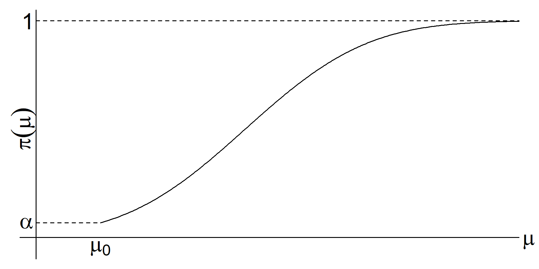
Figure 4.3: The power function, \(\pi(\mu),\) for the uniformly most powerful test of \(H_{0}: \mu = \mu_{0}\) versus \(H_{1}: \mu > \mu_{0}.\)

Some observations:

• For \(\mu=\mu_{0}\) we have \[\begin{eqnarray*} \pi(\mu_{0}) & = & 1 - \Phi(z_{1-\alpha}) \ = \ \alpha. \end{eqnarray*}\]
• As \(\mu\) increases, \(\Phi\left(\frac{\mu_{0} - \mu}{\sigma/\sqrt{n}} + z_{1-\alpha}\right)\) decreases so that \(\pi(\mu)\) is an increasing function which tends to 1 as \(\mu \rightarrow \infty.\)
• As \(\mu \rightarrow \mu_{0}\) it is very hard to distinguish between the two hypotheses.

4.3.2 Hypothesis testing for two-sided alternatives

We now consider testing for a so called two-sided alternative hypothesis, i.e. hypotheses of the form that \(\theta \neq \theta_{0}\) for some \(\theta_{0}.\) One approach is to combine the critical regions for testing the two one-sided alternatives.

Example 4.15 We consider that \(X_{1}, \ldots, X_{n}\) are i.i.d. \(N(\mu, \sigma^{2})\) with \(\sigma^{2}\) known. We wish to test the hypotheses \[\begin{eqnarray*} H_{0}: \mu = \mu_{0} & \mbox{ versus } & H_{1}: \mu \neq \mu_{0} \end{eqnarray*}\] We combine the two one-sided tests to form a critical region of the form \[\begin{eqnarray*} C & = & \{(x_{1}, \ldots, x_{n}): \overline{x} \leq k_{1} \text{ or } \overline{x} \geq k_{2}\}. \end{eqnarray*}\] For a test of size \(\alpha\) we must have \[\begin{eqnarray*} \alpha & = & P(\{\overline{X} \leq k_{1}\} \cup \{\overline{X} \geq k_{2}\} \, | \, \overline{X} \sim N(\mu_{0}, \sigma^{2}/n)) \\ & = & P\{\overline{X} \leq k_{1} \, | \, \overline{X} \sim N(\mu_{0}, \sigma^{2}/n)\} + P\{\overline{X} \geq k_{2} \, | \, \overline{X} \sim N(\mu_{0}, \sigma^{2}/n)\} \end{eqnarray*}\] One way to select \(k_{1}\) and \(k_{2}\) is to place \(\alpha/2\) into each tail as shown in Figure 4.4.

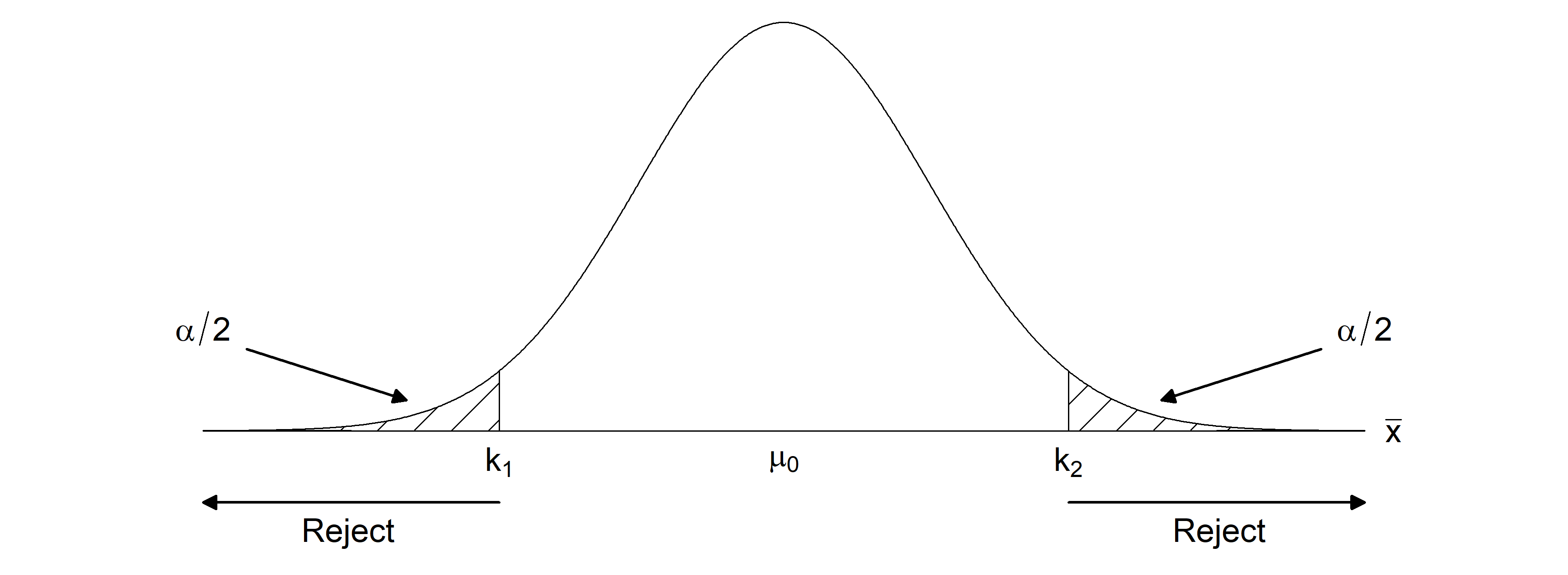
Figure 4.4: The critical region \(C = \{(x_{1}, \ldots, x_{n}): \overline{x} \leq k_{1} \text{ or } \overline{x} \geq k_{2}\}\) for testing the hypotheses \(H_{0}: \mu = \mu_{0}\) versus \(H_{1}: \mu \neq \mu_{0}\)

Then we have \[\begin{align*} k_{1} = \mu_{0} - z_{1- \frac{\alpha}{2}}\frac{\sigma}{\sqrt{n}},\quad \text{ and } \quad k_{2} = \mu_{0} + z_{1- \frac{\alpha}{2}}\frac{\sigma}{\sqrt{n}}. \end{align*}\] Thus, the test rejects for \[\begin{eqnarray*} \frac{\overline{x} - \mu_{0}}{\sigma/\sqrt{n}} \leq - z_{1- \frac{\alpha}{2}} & \mbox{ or } & \frac{\overline{x} - \mu_{0}}{\sigma/\sqrt{n}} \geq z_{1- \frac{\alpha}{2}} \end{eqnarray*}\] which is equivalent to \[\begin{eqnarray*} \frac{|\overline{x} - \mu_{0}|}{\sigma/\sqrt{n}} \geq z_{1 - \frac{\alpha}{2}}. \end{eqnarray*}\] Note that this test is not uniformly most powerful, since for any given simple hypothesis within the alternative, we can construct a one-sided test of size \(\alpha\) that is more powerful.

The corresponding power function is \[\begin{eqnarray*} \pi(\mu) & = & P(\mbox{Reject $H_{0}$} \, | \mu \neq \mu_0) \\ & = & P\{\overline{X} \leq k_{1} \, | \, \overline{X} \sim N(\mu, \sigma^{2}/n)\} + P\{\overline{X} \geq k_{2} \, | \, \overline{X} \sim N(\mu, \sigma^{2}/n)\} \\ & = & \Phi\left(\frac{\mu_{0} - \mu}{\sigma/\sqrt{n}} - z_{1- \frac{\alpha}{2}}\right) + 1 - \Phi\left(\frac{\mu_{0} - \mu}{\sigma/\sqrt{n}} + z_{1- \frac{\alpha}{2}}\right). \end{eqnarray*}\] The power function is shown in Figure 4.5. Notice that the power function is symmetric about \(\mu_{0}.\)

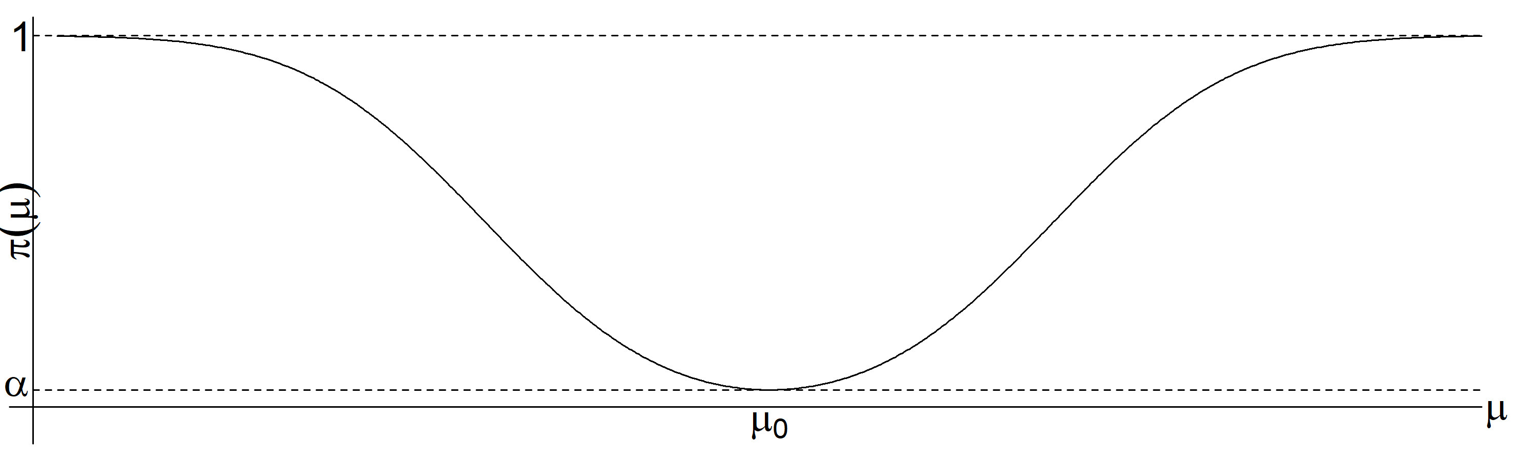
Figure 4.5: The power function, \(\pi(\mu),\) for the test of \(H_{0}: \mu = \mu_{0}\) versus \(H_{1}: \mu \neq \mu_{0}\).

4.3.3 Tests with unknown variance

Thus far we have considered tests for the normal mean when the variance \(\sigma^{2}\) is known. As we have noted previously, in practice it would typically not be known.

Example 4.16 Let \(X_1,\ldots,X_n\) be i.i.d. \(N(\mu,\sigma^2)\) where both \(\mu\) and \(\sigma\) are unknown. Consider the test of hypothesis \[H_0:\,\mu=\mu_0 \qquad\mbox{vs}\qquad H_1:\,\mu>\mu_0\] Because the variance \(\sigma^{2}\) is unknown and not specified by the two hypotheses, both hypotheses are composite, and we cannot apply the Neyman-Pearson Lemma.

In this case we cannot use the intuitive critical region \[C=\{(x_1,\ldots,x_n)\,:\, \overline{x}\geq k\}\] since when trying to find the value of \(k,\) we realize that we cannot compute \[P\left(\overline{X}\geq k|\mu=\mu_0 \right)\] based on \(\overline{X}\sim N(\mu,\sigma^2/n)\) because \(\sigma^2\) is now unknown. To construct a usable critical region we recall that under \(H_0\) \[T=\frac{\overline{X}-\mu_0}{S/\sqrt{n}}\sim t_{n-1},\] so that we can now define the critical region as \[C=\left\{(x_1,\ldots,x_n)\,:\,\frac{\overline{x}-\mu_0}{s/\sqrt{n}} \geq k\right\}.\] We can compute \(k\) since we can solve the following equation for \(k\) \[P\left(\frac{\overline{X}-\mu}{S/\sqrt{n}}\geq k | \mu=\mu_0\right)=\alpha\] for a given significance level \(\alpha.\) In fact, we clearly have that \(k=t_{n-1,1-\alpha}\) so that we reject when \[\begin{eqnarray*} \overline{x} \geq \mu_{0} + t_{n-1,1-\alpha} \frac{s}{\sqrt{n}} \end{eqnarray*}\] This test is known as the one-sided, one-sample t-test.

Example 4.17 Let \(X_1,\ldots,X_n\) be i.i.d. \(N(\mu,\sigma^2)\) where both \(\mu\) and \(\sigma^{2}\) are unknown. Consider the test of hypothesis \[H_0:\,\mu=\mu_0 \qquad\mbox{vs}\qquad H_1:\,\mu\neq \mu_0\] Since the \(t\)-distribution is symmetrical around zero, we can define a critical region as \[\begin{equation} C=\left\{(x_1,\ldots,x_n)\,:\,\left|\frac{\overline{x}-\mu_0}{s/\sqrt{n}}\right| \geq t_{n-1,1-\alpha/2}\right\} \tag{4.5} \end{equation}\] and this region has significance level \(\alpha.\) This test is known as the two-sided, one sample t-test.

Example 4.18 Let \(X_1,\ldots,X_n\) be i.i.d. \(N(\mu,\sigma^2)\) where both \(\mu\) and \(\sigma^{2}\) are unknown. Consider the test of hypothesis \[H_0:\,\sigma^{2}=\sigma^2_0 \qquad\mbox{vs}\qquad H_1:\,\sigma^2\neq \sigma^2_0\] Here we can use a result from Theorem 3.1 that \[\frac{(n-1)S^2}{\sigma_0^2}\sim \chi^2_{n-1}\] which is valid when \(H_0\) is true. Then we can use the critical region \[C=\left\{(x_1,\ldots,x_n)\,:\,\frac{(n-1)s^2}{\sigma_0^2} \leq k_1 \quad\mbox{or} \quad \frac{(n-1)s^2}{\sigma_0^2} \geq k_2\right\}\] where \(k_1<k_2.\) Then for a given significance level \(\alpha,\) we can take \(k_1=\chi^2_{n-1,\alpha/2}\) and \(k_2=\chi^2_{n-1,1-\alpha/2}\) since \[P\left(\left. \left\{\frac{(n-1)S^2}{\sigma_0^2}\leq k_1\right\}\cup \left\{\frac{(n-1)S^2}{\sigma_0^2}\geq k_2\right\} \right|\sigma^2=\sigma^2_0\right)=\] \[P\left(\left. \frac{(n-1)S^2}{\sigma_0^2}\leq \chi^2_{n-1,\alpha/2}\right|\sigma^2=\sigma^2_0\right)+P\left(\left. \frac{(n-1)S^2}{\sigma_0^2}\geq \chi^2_{n-1,1-\alpha/2}\right|\sigma^2=\sigma^2_0\right)=\frac{\alpha}{2}+\frac{\alpha}{2}=\alpha\]

4.3.4 Duality between Hypothesis Testing and Confidence Intervals

There is a close connection between hypothesis tests with two-sided alternatives and confidence intervals.

Example 4.19 Suppose \(X_{1},\dots,X_{n}\) are i.i.d. \(N(\mu,\sigma^{2})\) with \(\sigma^{2}\) known and we wish to test \(H_{0}:\mu=\mu_{0}\) versus \(H_{1}:\mu \neq \mu_{0}.\) Earlier we derived a test where we accept \(H_{0}:\mu=\mu_{0}\) if \[\begin{eqnarray*} \frac{|\overline{x} - \mu_{0}|}{\sigma/\sqrt{n}} < z_{1 - \frac{\alpha}{2}}. \end{eqnarray*}\] Equivalently, accept for \[\begin{eqnarray*} & -z_{1-\frac{\alpha}{2}} < \frac{\overline{x} - \mu_{0}}{\sigma/\sqrt{n}} < z_{1-\frac{\alpha}{2}} & \Leftrightarrow \\ & \mu_{0} - z_{1-\frac{\alpha}{2}}\frac{\sigma}{\sqrt{n}} < \overline{x} < \mu_{0} + z_{1-\frac{\alpha}{2}}\frac{\sigma}{\sqrt{n}} & \Leftrightarrow \\ & \overline{x}- z_{1-\frac{\alpha}{2}}\frac{\sigma}{\sqrt{n}} < \mu_{0} < \overline{x}+ z_{1-\frac{\alpha}{2}}\frac{\sigma}{\sqrt{n}} & \Leftrightarrow \end{eqnarray*}\] Recall, from the previous chapter (Equation (3.1)) that \((\overline{x}- z_{1-\frac{\alpha}{2}}\frac{\sigma}{\sqrt{n}}, \overline{x}+ z_{1-\frac{\alpha}{2}}\frac{\sigma}{\sqrt{n}})\) is a \(100(1-\alpha)\%\) confidence interval for \(\mu.\) We see that \(\mu_{0}\) lies in the \(100(1-\alpha)\%\) confidence interval if and only if the hypothesis test with Type I error \(\alpha\) accepts \(H_{0}.\) Conversely, the \(100(1-\alpha)\%\) confidence interval contains exactly those values of \(\mu_{0}\) for which we would accept \(H_{0}:\mu=\mu_{0}\) in the test with Type I error \(\alpha.\)

This shows a duality between the hypothesis test and the confidence interval: the latter may be obtained by inverting the former and vice versa. The duality in fact holds more generally.

Example 4.20 Suppose a 95% confidence interval of \((-1,3)\) has been calculated for the mean \(\mu.\) We can immediately deduce that we would not reject a two-sided hypothesis test of the null that \(\mu=0\) at level \(\alpha=0.05\) because the confidence interval includes zero. But we would reject a test of the null that \(\mu=4\) a \(\alpha=0.05\) level test, since \(4\) lies outside the 95% confidence interval.

4.4 P-values

The hypothesis testing approach we have described so far results in a binary decision or outcome: either reject or accept the null hypothesis \(H_{0}\). If the Type I error rate \(\alpha\) was set very small, rejection of the null is more convincing than if \(\alpha\) was set large. Apart from this however, the result of a hypothesis test is not very granular in regards to how strongly the null has been rejected, if it is rejected.

Example 4.21 Recall the drug testing example, Example 4.13. Suppose again that the study is conducted with \(\mu_{0}=10\), \(n=100\), \(\sigma=10\), and \(\alpha=0.025\). The critical value for testing \(\mu=\mu_{0}\) versus \(\mu>\mu_{0}\) is thus \[\begin{eqnarray*} \mu_{0} + z_{1-\alpha}\frac{\sigma}{\sqrt{n}} = 10 + 1.96 \frac{10}{\sqrt{100}} = 11.96 \end{eqnarray*}\] If the observed sample mean is \(\overline{x}=12\), we reject the null. If instead \(\overline{x}=15\), we again reject the null, but the binary decision of the test, on its own, gives no information about the strength of evidence against the null hypothesis. If in fact we had set \(\alpha=0.000001\), then the critical value would have been \[\begin{eqnarray*} \mu_{0} + z_{1-\alpha}\frac{\sigma}{\sqrt{n}} = 10 + 4.753 \frac{10}{\sqrt{100}} = 14.753 \end{eqnarray*}\] and so with \(\overline{x}=15\) we would have rejected at this much smaller significance level.

In the Neyman-Pearson hypothesis testing framework, the significance level / Type I error rate is fixed in advance, and cannot be modified upon seeing the data. In Sir Ronald Fisher’s testing framework, the p-value is a continuous measure of how compatible the observed data are with the null hypothesis.

The p-value can be viewed as the significance level at which the observed value of the test statistic would been on the accept/don’t recept borderline.

Definition 4.7 (P-value) Suppose that \(T(X_{1},\dots,X_{n})\) is our test statistic, such that the larger the value of \(T\) the stronger the evidence against \(H_{0}\) in favour of \(H_{1}\). Let \(t\) denote the observed value of \(T\). The p-value is defined as \[\begin{eqnarray*} p(t)=P(T \geq t | H_{0} \text{ true}). \end{eqnarray*}\]

The p-value measures the compatibility of the observed data (via the test statistic \(T\)) with the null hypothesis. It is therefore sometimes interpreted as measuring the evidence in the data against the null hypothesis: the smaller the p-value the stronger the evidence against the null hypothesis being true.

Simply put, the p-value can be viewed as the probability of observing a value at least as extreme as the observed data.

Example 4.22 Let \(X_{1}, \ldots ,X_{n}\) be i.i.d. \(N(\mu,\sigma^{2})\) with \(\sigma^{2}\) known, and consider testing \(H_{0}:\mu=\mu_{0}\) versus \(H_{1}: \mu>\mu_{0}\). In Example 4.12 we derived a uniformly most powerful size \(\alpha\) test for this setting which rejects \(H_{0}\) when \[\begin{eqnarray*} \overline{x} \geq \mu_{0} + z_{1-\alpha}\frac{\sigma}{\sqrt{n}}. \end{eqnarray*}\] Large values of \(\overline{x}\) are supportive of \(H_{1}\). Having observed \(\overline{x}\), the p-value is thus \[\begin{eqnarray*} P(\overline{X} \geq \overline{x} | H_{0} \text{ true}) &=& P\left(\overline{X} \geq \overline{x} | \overline{X} \sim N(\mu_{0},\sigma^{2}/n)\right) \\ &=& P\left(\frac{\overline{X}-\mu_{0}}{\sigma/\sqrt{n}} \geq \frac{\overline{x}-\mu_{0}}{\sigma/\sqrt{n}} | \overline{X} \sim N(\mu_{0},\sigma^{2}/n) \right) \\ &=& 1- \Phi\left(\frac{\overline{x}-\mu_{0}}{\sigma/\sqrt{n}} \right). \end{eqnarray*}\]

In the drug testing example (Example 4.21) with \(\mu_{0}=10\), \(n=100\), \(\sigma=10\) and \(\overline{x}=12\) we have \[\begin{eqnarray*} p(\overline{x} \geq 12) = 1 - \Phi\left(\frac{12-10}{10/10} \right) = 1-\Phi(2)=0.023. \end{eqnarray*}\] Since this value is less than 0.025, this agrees with our earlier finding that we reject \(H_{0}\) (just) if we test at \(\alpha=0.025\). The p-value enables us to deduce the result of the test for every significance level: for all tests of significance greater than 0.023 we reject \(H_{0}\). For all tests of significance less than 0.023 we do not reject \(H_{0}\).

If instead we had observed \(\overline{x}=15\), the p-value would have been \[\begin{eqnarray*} p(\overline{x}\geq 15) = 1 - \Phi\left(\frac{15-10}{10/10} \right) = 1-\Phi(5)<0.000001. \end{eqnarray*}\] In this case, either an incredibly rare event under \(H_{0}\) has occurred or the data does not support \(H_{0}\).

Example 4.23 Let \(X_{1}, \ldots ,X_{n}\) be i.i.d. \(N(\mu,\sigma^{2})\) with \(\sigma^{2}\) unknown, and consider testing \(H_{0}:\mu=\mu_{0}\) versus \(H_{1}: \mu>\mu_{0}\). In Example 4.16 we constructed a test for this situation which rejects when \[\begin{eqnarray*} \frac{\overline{x}-\mu_0}{s/\sqrt{n}} \geq t_{n-1,1-\alpha}. \end{eqnarray*}\] Here large values of \(t=\frac{\overline{x}-\mu_0}{s/\sqrt{n}}\) indicate support for the alternative hypothesis that \(\mu>\mu_{0}\). Having observed \(t\), the p-value is thus \[\begin{eqnarray*} P\left.\left(\frac{\overline{X}-\mu_0}{S/\sqrt{n}} \geq \frac{\overline{x}-\mu_0}{s/\sqrt{n}} \, \right| \, H_{0} \text{ true} \right). \end{eqnarray*}\] Under \(H_{0}\), \(T\) is distributed \(t_{n-1}\), and thus we have that the p-value is \[\begin{eqnarray*} P\left(T_{n-1} \geq \frac{\overline{x}-\mu_0}{s/\sqrt{n}}\right) = 1-P\left(T_{n-1} \leq \frac{\overline{x}-\mu_0}{s/\sqrt{n}}\right) \end{eqnarray*}\] where \(T_{n-1}\) is a random variable t-distributed on \(n-1\) degrees of freedom. This probability can thus be calculated using R or tables.

For two-sided tests we must be careful to calculate the p-value based on a test statistic for which large values indicate support for the alternative hypothesis:

Example 4.24 Let \(X_{1}, \ldots ,X_{n}\) be i.i.d. \(N(\mu,\sigma^{2})\) with \(\sigma^{2}\) unknown, and consider testing \(H_{0}:\mu=\mu_{0}\) versus the alternative \(H_{1}:\mu \neq \mu_{0}\). In Example 4.17 we derived a test for this setting which rejects when \[\begin{eqnarray*} \left|\frac{\overline{x}-\mu_0}{s/\sqrt{n}}\right| \geq t_{n-1,1-\alpha/2}. \end{eqnarray*}\] Large values of \(\left|\frac{\overline{x}-\mu_0}{s/\sqrt{n}}\right|\) indicate support for the two-sided alternative. Since the t-distribution is symmetric, the p-value is \[\begin{eqnarray*} P\left.\left(\left|\frac{\overline{X}-\mu_0}{S/\sqrt{n}} \, \right| \, \geq \left|\frac{\overline{x}-\mu_0}{s/\sqrt{n}}\right| \right| H_{0} \text{ true} \right) &=& 2 \times P\left(T_{n-1} \geq \left|\frac{\overline{x}-\mu_0}{s/\sqrt{n}}\right| \right) \end{eqnarray*}\] where \(T_{n-1}\) is t-distributed on \(n-1\) degrees of freedom.

If one has such a test statistic \(T,\) the p-value can be used to construct a valid size \(\alpha\) test of \(H_{0}\).

Theorem 4.1 The test which rejects \(H_{0}\) if and only if \(p(t) \leq \alpha\) is a valid test of significance/size \(\alpha\).

Proof: First write the p-value as \[\begin{eqnarray*} p(t)=P(T \geq t | H_{0} \text{ true})=1-F_{T}(t) \end{eqnarray*}\] where \(F_{T}(.)\) denotes the cumulative distribution function of \(T\) under \(H_{0}\). Then \[\begin{eqnarray*} P(p(T) \leq \alpha | H_{0} \text{ true}) &=& P(1-F_{T}(T) \leq \alpha| H_{0} \text{ true}) \\ &=& P(F_{T}(T) \geq 1-\alpha | H_{0} \text{ true}) \\ &=& P(T \geq F^{-1}_{T}(1-\alpha) | H_{0} \text{ true}) \\ &=& 1-F_{T}( F^{-1}_{T}(1-\alpha)) = \alpha. \end{eqnarray*}\] Thus the Type I error is controlled at \(\alpha\) as desired. \(\square\)

Hence, for all tests with significance level \(\alpha \geq p(t)\) we reject \(H_{0}\) and do not reject if \(p(t) > \alpha\).

If my observation \(t\) is such that I ject \(H_{0}\) at \(\alpha_{1}\) but do not reject at \(\alpha_{2}\) then \(\alpha_{1} > p(t) > \alpha_{2}\).

Notice, from the proof, that we have \(P(p(T) \leq \alpha | H_{0} \text{ true}) = \alpha\) so that the p-value has a uniform distribution on \([0, 1]\) when \(H_{0}\) is true.

4.4.1 Hypothesis testing and p-values - interpretation and recent controversies

The p-value is a continuous measure of strength of evidence against the null hypothesis, given the data, and assuming the model assumptions made are valid. A p-value less than 0.05 is conventionally reported as being ‘statistically significant’. Such phrasing has (particularly recently) been criticised, for many reasons, but partly because it is too easy to equate such a statement with the result being qualitatively/substantively significant.

The use of hypothesis testing and p-values in empirical research has in recent years come under quite a lot of criticism. In my view some of this is justified, but many of the problems discussed are more about the mis-interpretation or misuse by some of hypothesis tests and p-values, rather than intrinsic issues with the methodology. We shall not go through these here, except to mention perhaps the most striking incorrect interpretation of a p-value as being the probability that the null hypothesis is true.

If you are interested in reading more about this, see the following links, including the first with 25 misinterpretations of p-values, confidence intervals, and power:

• Statistical tests, P values, confidence intervals, and power: a guide to misinterpretations (2016)
• A Psychology journal bans P-values (2015)
• The American Statistical Association releases statement on the use of P-values (2016)

4.5 Robustness to model misspecification

We previously constructed tests that had size \(\alpha\) under the null hypothesis, for any sample size, under the assumed normal model. As we have discussed previously, a natural concern is whether our procedures are robust to certain misspecifications in the modelling assumptions. As for confidence intervals in Section 3.4, for certain tests we may be able to show that they would be robust to certain misspecifications as \(n \rightarrow \infty\). By robust, here we mean that their size, or Type I error probability, is maintained asymptotically at \(\alpha\) under the particular misspecification we are considering.

Example 4.25 (Robustness of z-tests and t-tests) We have previously considered the situation that \(X_{1}, \ldots ,X_{n}\) are i.i.d. \(N(\mu,\sigma^{2})\), and we are interested in tests for the mean \(\mu\). When \(\sigma^{2}\) is known, the test statistic for the z-test \[\begin{eqnarray*} Z=\frac{\overline{X}-\mu_0}{\sigma/\sqrt{n}} \end{eqnarray*}\] is distributed \(N(0,1)\) under the null \(H_{0}:\mu=\mu_{0}\). What if the normality assumption for \(X_{1}, \ldots,X_{n}\) does not hold? Is the Type I error rate controlled at level \(\alpha\)? From the Central Limit Theorem (Theorem 3.3) we know that, provided \(\text{Var}(X)\) is finite, without requiring the normality assumption, as \(n \rightarrow \infty\) \[\begin{eqnarray*} Z_{n}=\frac{\overline{X}_{n}-\mu_0}{\sigma/\sqrt{n}} \xrightarrow{L} N(0,1). \end{eqnarray*}\] under the null. As such, tests based on assuming \(Z \sim N(0,1)\) will continue to have the correct \(\alpha\) level asymptotically, even when the normality assumption for \(X_{1}, \ldots,X_{n}\) does not hold. For finite \(n\), how close the actual Type I error rate is to \(\alpha\) will depend on \(n\) and how far the true distribution is from the normal.

When \(\sigma^{2}\) is unknown, we previously derived the t-test, whose test statistic is \[\begin{eqnarray*} T=\frac{\overline{X}-\mu_0}{S/\sqrt{n}} \end{eqnarray*}\] which under the null \(H_{0}:\mu=\mu_{0}\) is t-distributed on \(n-1\) degrees of freedom. Now suppose we remove the normality assumption. Under the null that \(H_{0}=\mu=\mu_{0}\), provided \(\text{Var}(X)< \infty\) and \(S \xrightarrow{P} \sigma\), Slutzky’s Theorem gives \[\begin{eqnarray*} T_{n}=\frac{\overline{X}_{n}-\mu_0}{S/\sqrt{n}} = \frac{\overline{X}_{n}-\mu_0}{\sigma/\sqrt{n}} \times \frac{\sigma}{S} \xrightarrow{L} N(0,1) \times 1 = N(0,1) \end{eqnarray*}\] Thus again asymptotically the t-test will continue to have size \(\alpha\) even when the normality assumption for \(X_{1}, \ldots,X_{n}\) does not hold.

4.6 Summary of test statistics in the normal case

Let \(X_1,\ldots,X_n\) be i.i.d. \(N(\mu,\sigma^2).\)

• Investigating \(\mu\) when \(\sigma^2\) is known: z-tests \[z = \frac{\overline{x} - \mu_{0}}{\sigma/\sqrt{n}}\]

Table 4.2: Critical regions for one-sided and two-sided Normal tests (variance known).

\(H_0\)	\(H_1\)	Reject \(H_0\) if
\(\mu=\mu_0\)	\(\mu>\mu_0\)	\(z \geq z_{1-\alpha}\)
\(\mu=\mu_0\)	\(\mu < \mu_0\)	\(z \leq -z_{1-\alpha}=z_{\alpha}\)
\(\mu=\mu_0\)	\(\mu \neq \mu_0\)	\(|z| \geq z_{1-\alpha/2}\)

• Investigating \(\mu\) when \(\sigma^2\) is unknown: t-tests \[\displaystyle t=\frac{\overline{x}-\mu_0}{s/\sqrt{n}}\]

Table 4.3: Critical regions for one-sided and two-sided \(t\)-tests (variance unknown).

\(H_0\)	\(H_1\)	Reject \(H_0\) if
\(\mu=\mu_0\)	\(\mu>\mu_0\)	\(t \geq t_{n-1,1-\alpha}\)
\(\mu=\mu_0\)	\(\mu<\mu_0\)	\(t \leq -t_{n-1,1-\alpha}=t_{n-1,\alpha}\)
\(\mu=\mu_0\)	\(\mu \neq \mu_0\)	\(|t| \geq t_{n-1,1-\alpha/2}\)

• Investigating \(\sigma^2\) (\(\mu\) unknown): \(\chi^2\)-tests \[w=\displaystyle \frac{(n-1)s^2}{\sigma^2_0}\]

Table 4.4: Critical regions for one-sided and two-sided \(\chi^{2}\)-tests.

\(H_0\)	\(H_1\)	Reject \(H_0\) if
\(\sigma^2=\sigma^2_0\)	\(\sigma^2>\sigma^2_0\)	\(w \geq \chi^2_{n-1,1-\alpha}\)
\(\sigma^2=\sigma^2_0\)	\(\sigma^2<\sigma^2_0\)	\(w \leq \chi^2_{n-1,\alpha}\)
\(\sigma^2=\sigma^2_0\)	\(\sigma^2\neq\sigma^2_0\)	\(w \geq \chi^2_{n-1,1-\alpha/2}\)
		or \(w \leq \chi^2_{n-1,\alpha/2}\)