Calculating tnt solvation with Gromacs¶

Carmelo Herdes <c.e.herdes.moreno@bath.ac.uk>, Claire Hobday <c.l.hobday@bath.ac.uk> and Gaël Donval <g.donval@bath.ac.uk>

In this tutorial you will build on your molecular dynamics simulations skills and use Gromacs in conjuction with other computational tools to build up a simulation cell from scratch to investigate the effects of temperature on the solvation of $2,4,6\mathrm{-trinitrotoluene}$ (tnt) in water.

Objectives

Enhancing practical understanding of molecular dynamics simulations.
Learning how to use MarvinSketch to build 3-D models of molecules for molecular dynamics input.
Learning how to use MkTop to create a topology and force field input for molecular dynamics.
Learning how to run molecular dynamics simulations using the program Gromacs on the university’s high performance computing cluster, Balena.
Learning how to visualize results using Vmd.
Using molecular dynamics to work in different statistical ensembles, e.g. nvt and npt simulations.

Before you start:

Review the slides on molecular dynamics simulations.
Be sure you can access Balena.

Background¶

Nowadays complicated problems are often simulated using computers for three basic reasons: to minimize human error, to avoid time constraints and to save money. Different programs are used everyday and everywhere depending on the field, application, and desired simulation, ranging from the quantum level up to the cosmological scale (e.g. the Illustris project is a large cosmological simulation of galaxy formation).

Over the course of this tutorial, you will be introduced to some of the (basic) features of MarvinSketch, MkTop, Gromacs and Vmd to build up a simulation cell from scratch and to investigate the effects of temperature on the solvation of tnt in water. These off-the-shelf programs are very powerful common tools in the field of molecular simulation.

Let’s start!

Drawing your tnt molecule¶

MarvinSketch is an advanced chemical editor for drawing chemical structures, queries and reactions. It allows you to quickly draw molecules through basic functions on the screen and advanced functionalities such as sprout drawing, customisable shortcuts, abbreviated groups, default and user-defined templates and context-sensitive popup menus.

It should be available on the university computers. To install it on own your computer, go to the ChemAxon website. Click on download and select the relevant version for you (note that a portable version is provided under the Platform Independent section).

Once installed/copied over, open MarvinSketch and familiarise yourself with the canvas window (see Fig. 3); hover over the various items and toolbars to see what you can do!

Fig. 3 MarvinSketch’s canvas is where you can draw molecules.¶

Once you are familiar with the interface, you can start building your target molecule, tnt, following its representations in Fig. 4.

Fig. 4 tnt chemical structure and 3D atomistic model. Source.¶

There are actually many ways of drawing that molecule in MarvinSketch. None of them are intrinsically better but we suggest that you start by using building elements that are the closest possible to the final structure you want to represent. In this case, we could start by inserting a benzene ring by clicking on the benzene ring symbol at the left of the bottom toolbar. Then place it on the canvas by clicking anywhere and press Esc (to avoid placing any more of them next time you click on the canvas).

Then create new methyl groups ($\mathrm{CH}_3$) by selecting and using the Single bond tool (top of the left toolbar) until you get a structure similar to what is depicted in Fig. 5. Once finished, remember to press Esc to unselect the current tool.

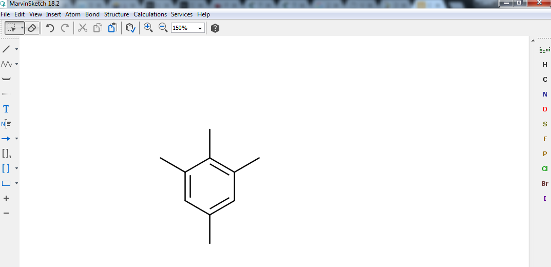
Fig. 5 Benzene ring with four extra methyl groups ready to be edited. Note that, by default, hydrogen atoms are not displayed: each dangling bond is actually a $\mathrm{CH}_3$ in disguise!¶

But as you can see back in Fig. 4, only one group should actually be a $\mathrm{CH}_3$. The rest should be made of nitro groups ($\mathrm{NO}_2$) instead! Fortunately, MarvinSketch allows you to change the chemical nature of any atom you want. Have a look at the toolbar at the right of your screen, click on N. Now hover your pointer over the carbon atoms you would like to replace by nitrogen and click to make the substitution. Repeat until you get the result shown in Fig. 6.

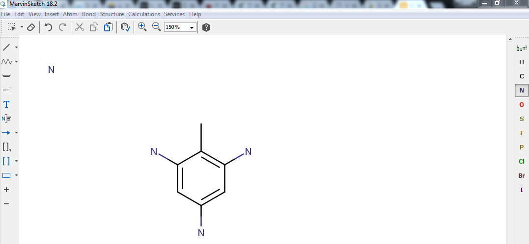
Fig. 6 The result of the substitution of the methyl groups by nitrogen.¶

Now it will be easier if we could see all the hydrogen atoms that were kept hidden until now. To do so, click Structure ‣ Add ‣ H Explicit Hydrogens. Then perform the required substitution of hydrogens to oxygens to transform the amino groups ($\mathrm{NH}_2$) to nitro groups.

Finally, you must convert the single bonds between the oxygens and nitrogens into double bonds. To do so, click on the small arrow at the right of the Single bond tool (top of the left toolbar), select the Double bond tool and click on the single bonds you need to convert.

The final structure is shown in Fig. 7. Check carefully that you obtained the same result.

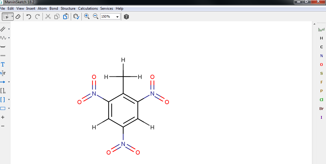
Fig. 7 TNT 2D model.¶

The very last step before saving that structure is to make it 3D! Select Structure ‣ Clean 3D and you should get a 3D structure that you must save (File ‣ Save) as a protein data bank (.pdb) file: TNT.pdb. We suggest that you try opening this structure in Vmd to really see that the structure you generated seems proper.

Congratulations! You have just created your first structure from scratch. You are now ready to set up your molecular dynamics simulation.

Converting tnt into the Gromacs format¶

First we need to convert the structure file TNT.pdb into a structure file readable by Gromacs: TNT.gro. As before, we are providing you with a few files to help you setting your working environment up. Download, copy and extract them into a relevant directory (e.g. ~/scratch/tutorials/gromacs) from this link: TNT.tar.xz.

$ tar -xf TNT.tar.xz

Locate the newly created directory and create two copies of that folder: TNT_NVT and TNT_NPT:

$ cp -r TNT TNT_NPT
$ mv TNT TNT_NVT

Go into TNT_NVT and copy over the file TNT.pdb that you have just created with MarvinSketch into that directory. As usual when we need to do any actual work, we need to log into a computing node and load Gromacs:

$ sint
$ module load gromacs/2019.2

Then edit the TNT.pdb file you have just created and replace all the instances of UNK by TNT: this is a way of specifying that all the atoms in that file belong to a Gromacs group (here, a molecule) called TNT. That name would usually be arbitrary: you would just need to find something descriptive. In this specific case though, TNT is also used in other files we provided (most notably system.top): so you need to stick to it.

Hint

The easiest way to do so in nano is to use its find-and-replace feature: press Ctrl-\ then type UNK as a search token, replace with TNT and press a to replace all occurrences at once or y to validate each line.

Then convert that .pdb file to a .gro file:

$ gmx editconf -f TNT.pdb -o TNT.gro

You can have a look at the generated TNT.gro file. It contains information about the type and position of each atom.

Defining force-fields¶

Gromacs now has a structure to work with but if you remember the introductory lecture about molecular simulations, you also need to provide Gromacs with information about how each atom interacts with each other: you need to define force-fields.

Gromacs already contains extensive lists of parameters. You are going to use the opls-aa set (optimized potential for liquid simulations all atoms). However Gromacs does not know that. Neither does it know how you intend to use them exactly: you need to write a topology file (.itp) to do that.

Such a file must contain:

A list of all the atoms in the molecule, their atom type, their mass and charge.
A list of bonds: a list of what atom numbers are bonded to each other plus a flag to describe the kind of bond (i.e. which sort of force-field to use, e.g. 1 for a harmonic potential).
A list of angles: like bonds, but three atom numbers are needed.
A list of dihedrals (including improper dihedrals where appropriate): four atoms numbers must be specified.
The 1,4 pairs: a list of pairs of atoms numbers.

Defining such a file would most likely take days. In practice, .itp topology files can often be readily found alongside publications or in databases. In our case we are going to create that file nonetheless with the help of a small program, MkTop (make topology).

That program should already be in your tutorial folder:

$ ./mktop -i TNT.pdb -o TNT.itp -ff opls -conect no

The -ff opls flag specifies that the opls-aa force-field should be used; The -conect no flag tells MkTop that our .pdb file does not contain any bond information (this is not included in output files from MarvinSketch).

Getting your topology file right¶

In a perfect world, the ./mktop command above would be enough to get a working TNT.itp file… but it isn’t. The file TNT.itp needs some editing:

Under [ moleculetype ], change the name of the molecule from MOL to TNT.
Under [ atoms ], remove the numbers after each atom symbol. For instance C1 should become C, C2 should become C as well, etc.
Still in the [ atoms ] section, you must set each of the atom’s charge by its proper value (currently they are all set to 0.00000). To do so,
- make a note of each atom type (i.e. the names starting by opls_);
- open oplsaa.ff/ffnonbonded.itp (with less): that file contains all the force-fields parameters Gromacs will be using;
- find each entry corresponding to each atom type you identified in TNT.itp;
- find the charge corresponding to each entry;
- replace each charge in TNT.itp by its proper value.
Hint

Use / to search for something less. Use n to jump to the next matching element or Shift-n to get back to the previous one.

Remove the following unneeded lines from the end of TNT.itp:

[system]
; Name
MKTOP

[ molecules ]
; Compound       #mols
MOL           1

From Gromacs’s perspective, the atom type (starting with opls_) is a reference to the force-field parameters found in the database file oplsaa.ff/ffnonbonded.itp. MkTop cannot read that file though to copy charges over: this is why you had to do it yourself.

A human-readable description of each type is also provided in oplsaa.ff/atomtypes.atp: have a look at it and make sure the atom types in TNT.itp look right.

Checking your topology¶

The best way to quickly find if there is something really wrong in your system is to calculate its total charge: just sum all the partial charges you have set in TNT.itp. Do they add up to zero? Why do you expect that system to be neutral? What would happen if the system weren’t neutral (think about periodic boundary conditions)?

In principle, you should also check for consistency using indications in oplsaa.ff/atomtypes.atp: e.g. if one of your nitrogens were of a type opls_145 described as Benzene C in oplsaa.ff/atomtypes.atp, something would be really wrong somewhere. However doing a full manual check with oplsaa.ff/atomtypes.atp and Vmd would take too much time in the span of this tutorial: we have already checked that MkTop behaves correctly with tnt.

Attention

Should you want to do that consistency check yourself, be aware that Vmd start counting from 0 while atoms are referenced from 1 in TNT.itp. This means that what Vmd identifies as atom 0 is actually the atom of index 1 in TNT.itp while atom 1 in Vmd is actually at index 2 in TNT.itp, etc.

Preparing the simulation box¶

If we really wanted to follow the aforementioned paper we would need to simulate the behaviour of $50\,\mathrm{mg}$ of tnt into $1\,\mathrm{L}$ of water at $35\,\mathrm{ºC}$ and $1\,\mathrm{bar}$. What usually really matters though is not absolute quantity of components but concentrations. So the real question is how many molecules of tnt and water do we need to place in a given simulation cell to reach such a concentration?

Knowing that tnt molecular weight is $227.13\,\mathrm{g/mol}$ and water density in these conditions is $55.177\,\mathrm{mol/L}$ we find that we need about 250 thousand water molecules per tnt molecule. Do you think this kind of system size can be reached in practice? Is it worth trying it? If you have no idea, try to roughly extrapolate from the execution time you had when calculating bulk water properties.

Anyway, such a system cannot be studied in the remaining time of this tutorial. We are going to create a much simpler system instead: 10 tnt molecules in a simulation box containing 1000 water molecules. We are going to proceed in two steps:

We need to insert our tnt molecules into a simulation box (here $5^3\,\mathrm{nm}^3$):
```
$ gmx insert-molecules -ci TNT.gro -box 5 -nmol 10 -o 10TNT.gro
```
Here, gmx insert-molecules is the Gromacs sub-command used to insert molecules in a simulation box; -ci specifies the structure of the molecule that must be inserted; -box sets the size of the simulation box in nanometres (if only one number is given, Gromacs just assumes the system is cubic); -nmol sets the number of molecules to add and -o specifies the name of the output file.

By all mean, visualise your 10 tnt molecules (10TNT.gro) in Vmd!
Now we need to add the 1000 water molecules in the box as well:
```
$ gmx solvate -cp 10TNT.gro -cs -maxsol 1000 -o TNT_Water.gro
```
Here, gmx solvate is the solvation sub-command; -cp specifies the box we want to solvate; -cs specifies the the solvent we want to insert, -maxsol sets the number of solvent molecules to add and -o redirects the output into a file called TNT_Water.gro.

Visualise the output in Vmd and type the following (in Vmd terminal) to visualise periodic boundary conditions on your simulation cell:

$ pbc box

Do you see why we did not start by adding the water and then add the tnt molecules in?

Running the simulation¶

We are finally ready to run the simulation! We could execute the following if we are still on a computing node (but wait, don’t do it):

$ gmx grompp -v -f NVT.mdp -c TNT_Water.gro -o topo.tpr -p system.top
$ gmx mdrun -v -s topo.tpr -c TNT_Water.gro

However this is going to take hours! Since the beginning, we have been using computing nodes directly: they are nice but limited (you can’t ask for more than one node at once, you can only stay on it 6 hours at a time, you cannot disconnect without killing your job). We should instead employ an automated approach to running our jobs.

The usual way of requesting computing resources on Balena consists in submitting so-called submission scripts. In our case, such a submission script has been provided: TNT.sbatch. You can read more about that file in How do you submit a job?.

That file can be submitted to the job scheduler using:

$ sbatch TNT.sbatch

Note

If you are a project student in you training week, you can change the following lines:

#SBATCH --account=free
#SBATCH --partition=batch

into those ones to get a faster access to resources:

#SBATCH --account=ce30122
#SBATCH --partition=teaching

Warning

Don’t play with TNT.sbatch in general: computing resources are accounted for and an overuse would make further submissions more difficult.

That file is going to request resources for your job and execute Gromacs in parallel on multiple cpu cores: instead of having to wait for hours, the calculation should terminate within 30 minutes.

You can review what you have submitted using:

$ squeue -u <username>

Once your job is running (i.e. the ST column should show R), you can follow its state in slurm-*.out (again * in that context is a wildcard). You can open it with less and press Shift-f to display the data as it comes in.

One a job is submitted like this, don’t change anything related to its working directory anymore: don’t rename, move, edit, change or copy anything.

Exercises¶

The simulation you are running is performed in the nvt ensemble (you should see that a thermostat is set in NVT.mdp, Tcoupl). It is going to take around 20 minutes to finish (unless you made a mistake somewhere).

In the meantime, go in the other copy of the directory you created right at the beginning:

$ cd ../TNT_NPT

Rename (mv) NVT.mdp to NPT.mdp and edit the file to use berendsen barostat (Pcoupl). Edit TNT.sbatch to use NPT.mdp instead of NVT.mdp. Copy the required files from ../TNT_NVT to avoid having to go through the whole manual editing process again. Finally submit that new job to Balena.

Once the nvt simulation is run, visualise the molecular dynamics trajectory (with Vmd) and use the post-processing commands you saw in Calculating properties of water with Gromacs. When is your system equilibrated? Have a look at the time evolution of temperature: is it what you expected?

Finally, calculate the density of your system using the results from the npt simulation.

Have a nice simulation!