Calculating Henry’s coefficients with Raspa

Matthew Lennox <m.j.lennox@bath.ac.uk> and Gaël Donval <g.donval@bath.ac.uk>

In most adsorption applications, we are interested in the capacity of a material (i.e. how much sorbate it will adsorb) and the affinity of the material for a given species (i.e. how strongly the sorbate is adsorbed). This information is often presented in the form of an adsorption isotherm (i.e. how much gas is adsorbed in a material with respect to external pressure).

In later sessions, you will use Monte-Carlo simulations to predict and investigate the full adsorption isotherm. In this tutorial, you will focus on one particular way of quantifying the affinity of a material for a given species: Henry’s coefficient.

Objectives

1. Becoming more familiar with Linux and the Hpc facilities, running simulations using Raspa (a multipurpose Monte-Carlo code) and using Vmd.

2. Acquiring a basic understanding of how Henry’s coefficient relates to the adsorption isotherms and to certain applications.

3. Beginning to explore how molecular-level information relates to the adsorption process and some of the characteristics and properties which influence adsorption in porous solids.

Before you start:

1. Review the slides on Monte-Carlo simulations.

2. Optionally read the introductory chapter in Rouquerol, Adsorption by Powders and Porous Solids, for a brief introduction to key concepts in adsorption.

Background

You may have encountered Henry’s Law already in relation to the solubility of a gas in a liquid, or the volatility of a liquid. In studies of adsorption, Henry’s coefficient (\(K_\mathrm{H}\)) is an indicator of the strength of interaction between the sorbate and the adsorbent at infinite dilution (i.e. when very few adsorbed molecules are present in the system). It is related to the slope of the initial, linear, portion of an isotherm as illustrated in Fig. 8. The steeper the slope, the greater the value of \(K_\mathrm{H}\) and the more strongly adsorbed the species is.

Fig. 8 Full adsorption isotherm: as the pressure increases, the porous material’s gas uptake also increases; more gas is adsorbed at higher pressure. In the limit of vanishing pressures, the quantity of adsorbed gas is proportional to pressure itself. The slope of the resulting straight line is Henry’s coefficient \(K_\mathrm{H}\).

\(K_\mathrm{H}\) is dependent on the temperature of the system as well as the composition and characteristics of both the sorbate and adsorbent. It is a useful indicator for applications in which the low pressure (low loading) portion of an isotherm is important, e.g. detecting or removing a harmful compound at low concentration in water (or in air).

The selectivity of a material for one compound over another (i.e. how easy it would be to separate two compounds via adsorption) can also be estimated from the ratio of their respective \(K_\mathrm{H}\) values.

In principle \(K_\mathrm{H}\) should be extracted from a full isotherm calculation. However at vanishing pressures the system is effectively in an infinite dilution state: the adsorbed gas molecules are so few that they don’t “see” each other. Their being non interacting can be efficiently leveraged using a specific Monte-Carlo technique, Widom insertion, that does not require a full isotherm calculation.

In this method, we are interested in evaluating the interaction energy of one adsorbed molecule with the adsorbent. The molecule is inserted at a random location in the simulation box, the interaction energy is calculated and the molecule is then removed. This is repeated for many thousands of trial points, allowing us to calculate the average interaction energy for the molecule-adsorbent system. Since we only considered one adsorbed molecule at any step, this is essentially adsorption at an extremely low loading, so can be related to the Henry’s coefficient via some thermodynamic relationships.

You will use Widom insertion in this tutorial to estimate \(K_\mathrm{H}\) for \(\mathrm{CO}_2\), \(\mathrm{H}_2\mathrm{O}\) and tnt in two different metal-organic frameworks (mofs) at room temperature.

Preparing the simulation

Start by logging in on the cluster if you are not on it already. Create a new folder such as ~/scratch/tutorials/raspa. Download the required files from this link: IRMOF1.tar.xz, copy them into that new ~/scratch/tutorials/raspa folder and uncompress it it:

$ tar xf IRMOF1.tar.xz

Have a look at the newly created folder, go into it and look into the files (using less):

• CO2.def, TNT.def and Tip5p.def are all molecule definition files: they specify the types of atoms (or pseudo-atoms) present in the molecule and their relative positions. Why do you think TNT.def only contains 16 ‘atom’ groups? Why do you think water (Tip5p.def) contains five?

• IRMOF1.cif is also a molecule definition file. This one specifies the type and positions of atoms for Irmof-1.

• pseudo_atoms.def defines some properties of all of the atoms and pseudo-atoms used in the simulation. You won’t need to change anything in here.

• force_field_mixing_rules.def and force_field.def define the force field parameters used for the simulation (Lennard-Jones in this case).

• simulation.input is what tells Raspa what type of simulation we want to carry out. This is the file we will be focusing on.

We greatly encourage you to inspect the structure of Irmof-1 using Vmd. We provide an illustration in Fig. 9 but you should get a better feeling of what it really looks like if you can move it around.

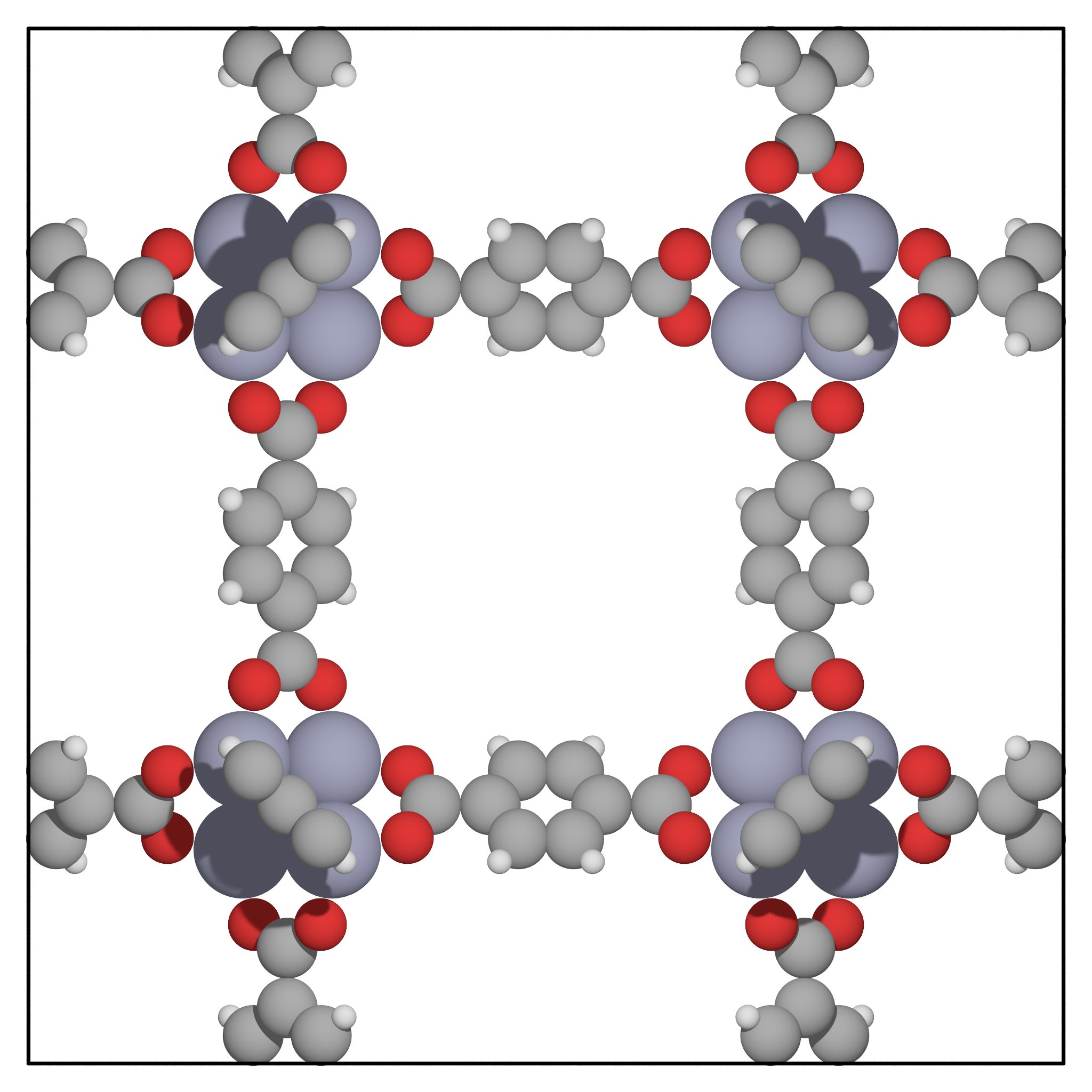
Fig. 9 Picture of Irmof-1: this is a porous metal-organic framework (mof); it can accomodate molecules in its midst. How exactly it does so is captured in its adsorption isotherms, where the quantity of guest molecules is plotted against external pressure.

The file simulation.input can be divided into three parts.

Lines 1 to 8 in List. 3 correspond to the first part, where you must define the kind of simulation you want to carry out. The most important parameters are NumberOfCycles which is related to the number of Monte-Carlo moves we will perfom: the higher the number, the longer the simulation; ChargeMethod which is set to None meaning we are ignoring electrostatic interactions and CutOffVDW which defines a cut-off radius of \(12.8\,\mathrm{Å}\) for Lennard-Jones interactions. At the moment, we have chosen a nonsensically small number of cycles: this is going to be changed when we run our first calculations. Now think about the molecules we are simulating: do you think electrostatics are important in these cases? Why do you think we have ignored them for this 2-hour workshop?

List. 3 ~/scratch/tutorials/raspa/IRMOF1/simulation.input

SimulationType                MonteCarlo
NumberOfCycles                2
NumberOfInitializationCycles  0
PrintEvery                    1000
PrintPropertiesEvery          1000
Forcefield                    raspa
ChargeMethod                  None
CutOffVDW                     12.8

Framework 0 
            FrameworkName                 IRMOF-1
            RemoveAtomNumberCodeFromLabel no
            UnitCells                     1 1 1
            ExternalTemperature           298.0

Component 0 MoleculeName                  CO2
            MoleculeDefinition            local
            IdealRosenbluthValue          1.0
            WidomProbability              1.0
            CreateNumberOfMolecules       0

Component 1 MoleculeName                  TNT
            MoleculeDefinition            local
            IdealRosenbluthValue          1.0
            WidomProbability              1.0
            CreateNumberOfMolecules       0

Component 2 MoleculeName                  Tip5p
            MoleculeDefinition            local
            IdealRosenbluthValue          1.0
            WidomProbability              1.0
            CreateNumberOfMolecules       0

The second part starts on line 10 with the definition of the porous framework Framework 0 wherein we are going to do our calculations. We told Raspa to use the structure given in IRMOF-1(.cif) and to thermalise it at \(298.0\,\mathrm{K}\). Irmof-1 is a crystal: it is defined in term of a repeating unit called a unit-cell. That unit-cell is actually a box: by specifying UnitCells  1 1 1 we are simply telling Raspa that our whole simulation box should be as big as a single unit-cell along the \(x\), \(y\) and \(z\) directions (we will come back to this later).

The third part starts on line 16 in this example and encompasses all the gas molecules Component n that we want to use for Widom insertion. The MoleculeName refer to each respective .def file. For a usual calculation, specifying multiple components at once like this would mean we want to study a mixture of them. However because Widom insertion does not actually insert anything, we can evaluate \(K_\mathrm{H}\) for all three components at once!

Running the simulation for Irmof-1

We remind you that running simulations on Balena, directly in the command line, is strictly forbidden. When you are on Balena, you log onto the front node. This is used for general accessing of files and folders, but not anything which requires great computing power. As we did before, we are going to log onto a computing node using a script that we provided:

$ sint
$ module load raspa/2.0.2

If logging on the node was successful, you should see a green name appearing on the prompt. A new command, simulate will also be made available. This command allows you to run Raspa for this example.

Warning

Though tempting, don’t submit Raspa jobs with sbatch as you saw in the previous section: this would be wasting resources for absolutely no gain, as Raspa is not a parallel code. The proper way to submit Raspa jobs is by using Taskfarmer as we will explain in Leveraging full nodes using Taskfarmer.

Edit simulation.input and set the number of cycles to 20, save and close the file. Then run the simulation:

$ simulate simulation.input

The simulation should last a few seconds. Once it is finished, you will see several new directories. The simulation results are stored in Output/System_0/. Use ls to see which file is in there. That file is quite big. We are going to use grep to filter out the output file and only display Henry’s coefficients:

$ grep "Average Henry" Output/System_0/output_*
Average Henry coefficient:
  [CO2] Average Henry coefficient: XXX +/- XXX
  [TNT] Average Henry coefficient: XXX +/- XXX
  [Tip5p] Average Henry coefficient: XXX +/- XXX

We can do the same for adsorption energies, the average strength of interaction between the compound and the mof:

$ grep "kJ/mol)" Output/System_0/output_*

Do the same calculation for each of these numbers of cycles: 20, 100, 200, 1000, 2000. Note down \(K_\mathrm{H}\) and the adsorption energies for each of them. Also appreciate how, as you increase the number of cycles, the calculation takes longer and longer to terminate. Which \(K_\mathrm{H}\) exhibits the most variation? Why?

Have a look at the adsorption energies. Did you expect the interaction energy to be negative or positive for adsorption?

Hint

For long file names such as the one used by Raspa for its output, it is really convenient to get some help from the prompt instead of copy-pasting the output of ls. One trick is to use Tab to auto-complete the current file name (one for auto-completion, two for displaying matching file names):

$ grep "Average Henry" Output/System_0/out{Tab}{Tab}

The other way (used above) is to type a * (pronounced wildcard) to tell the prompt to provide the program with all inputs matching (i.e. starting with) Output/System_0/output_.

Running the simulation for UiO-66

Now let’s try calculate Henry’s coefficients for the same molecules in a different mof: UiO-66. Download the .cif file from here: UiO66.tar.xz. Copy it over to ~/scratch/tutorial/raspa (or whichever folder you have chosen). Decompress it and go in:

$ tar xf UiO66.tar.xz

Again, use Vmd to familiarise yourself with this new structure. A picture of it is given in Fig. 10 but you should use the viewer to understand its pore geometry.

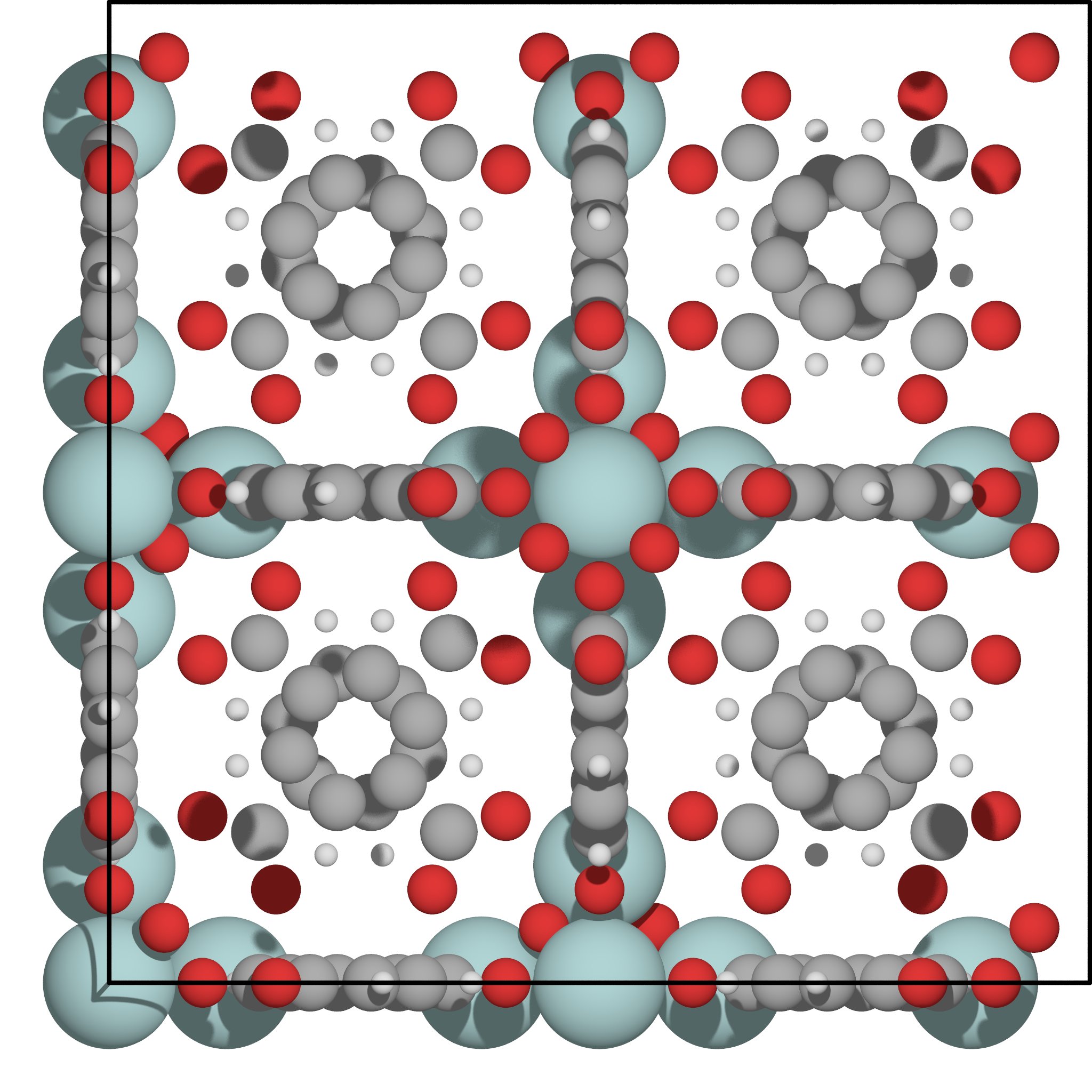
Fig. 10 Picture of UiO-66: just like Irmof-1, this is a porous metal-organic framework; it can accomodate molecules in its midst. Note how different its pore geometry is from Irmof-1.

This time you only have the .cif file at your disposal. You could type in everything from scratch, but we suggest instead that you copy over the files from your previous calculations in the current folder. You can use the wildcard pattern discussed above to select all the files from ~/scratch/tutorials/raspa/IRMOF1/ at once.

What needs to change in simulation.input? Be sure to use the correct framework name.

There is one other thing that needs to be changed. Like Irmof-1, the unit-cell of UiO-66 is cubic but it is only \(20.7\,\mathrm{Å}\) along each edge (Irmof-1 has edge lengths of \(25.8\,\mathrm{Å}\)). We are using a cut-off radius of \(12.8\,\mathrm{Å}\). Is a simulation box of \(1\times 1\times 1\) UiO-66 unit-cell big enough (recall the minimum image convention from molecular dynamics lecture)? Should you increase the number of unit-cells or should you decrease the cut-off radius?

Once you are confident about the changes you made, be absolutely certain to still be on the computing node and launch the calculation as described before. Once finished, make a note of the average \(K_\mathrm{H}\) and interaction energy for each compound.

Analysing the data

• You should start by comparing the average \(K_\mathrm{H}\) obtained for each compound in Irmof-1: which one is the most strongly adsorbed? how does this relate to adsorption energies?

• Take each compound one by one and compare adsorption energies for each framework: is one framework more strongly-interacting than the other? What about \(K_\mathrm{H}\)? One of the most important factors in adsorption in microporous adsorbents (solids which have pores \(< 20\,\mathrm{Å}\) in diameter) like Irmof-1 and UiO-66 is the pore size. Generally, molecules are more strongly adsorbed in smaller pores. Why do you think this is the case? Do your results agree with this general trend?

  To answer these questions, you need to estimate pore sizes. For the time being, you can get a fairly good estimation of it in Vmd by measuring the distance between atoms using the Mouse ‣ Label ‣ Bonds menu and by clicking on any two atoms to get a distance (even if they are non-bonded to each other). If you chose appropriate atoms, you should be able to get a rough estimate of pore diameters for each structure.

• In most applications, more than one compound will be present in the process. For both \(\mathrm{CO}_2\) capture (where we try to remove \(\mathrm{CO}_2\) from flue gases) and tnt detection, water will be present in the process. We want to selectively adsorb \(\mathrm{CO}_2\) or tnt and adsorb as little water as possible. You can use Henry’s coefficients to estimate the selectivity \(S_\mathrm{ab}\) between species \(\mathrm{a}\) and \(\mathrm{b}\) at low loading:

  \[S_\mathrm{ab} \approx \frac{K_\mathrm{H}^\mathrm{a}}{K_\mathrm{H}^\mathrm{b}}\]

  A selectivity of greater than \(1\) indicates that component a will be preferentially adsorbed. Based on your results, which mof is a better choice for use in a carbon capture process? What about tnt detection?

• What about equilibration in this case? How many values should we remove to get a good sample?

Going further

In this tutorial we have used the TraPPE (transferable potentials for phase equilibria) models for \(\mathrm{CO}_2\) and tnt. These parameters are fitted against experimental vapour-liquid equilibria data in the case of \(\mathrm{CO}_2\). For tnt, those data don’t exist and so the parameters are those developed for similar compounds.

Note

It is always a good idea (read, necessary) to identify limitations in your simulation approach!

Instead of the spc water model you used earlier, we are using a slightly more complicated model (tip5p). The dispersion interactions are still modelled using a Lennard-Jones potential based solely on oxygen–oxygen interactions, but there are some extra pseudo-atoms (called Lw in this simulation) with electrostatic contributions to try and model the hydrogen bonding more effectively than spc water. For more detail on the concepts, thermodynamics and maths behind Henry’s constants as applied to adsorption, you may find Rouquerol’s Adsorption by Powders and Porous Solids helpful, as well as Myers’ Thermodynamics of Adsorption (though it is a bit more heavy-going than the former).