Calculating properties of water with Gromacs¶

Tina Düren <t.duren@bath.ac.uk>, Lev Sarkisov <Lev.Sarkisov@ed.ac.uk>, Gaël Donval <g.donval@bath.ac.uk> and Claire Hobday <c.l.hobday@bath.ac.uk>

In this tutorial you will use molecular dynamics simulations to investigate the thermodynamic properties and structural characteristics of bulk water using a molecular simulation package called Gromacs.

Objectives

Acquiring basic practical understanding of molecular dynamics simulations.

Learning how to run molecular dynamics simulations using the program Gromacs on the university’s high performance computing cluster, Balena.

Learning how to visualize your results using Vmd.

Learning about basic molecular models of water; fundamental properties of water, role of hydrogen bonds in the unusual behaviour of water.

Familiarizing yourself with key concepts of molecular modelling such as radial distribution functions and self-diffusion coefficient from mean squared displacement of molecules as function of time.

Before you start:

Review the slides on molecular dynamics simulations.
Review your command-line notes.
If you have access to the book, read chapter 29 of Dill and Bromberg, Molecular Driving forces, on water properties.
Test yourself by answering the following questions:
- What is the geometry of a water molecule?
- What is a hydrogen bond? How do we know that two water molecules formed a hydrogen bond? What is the strength of a hydrogen bond? How many hydrogen bonds does a single molecule of water form on average in liquid water at ambient conditions?
- What are the anomalous properties of water compared to other liquids (such as liquid argon or methane)?

Background¶

Properties of water are of an immense importance in both biology and various technological applications, and at the same time they exhibit a number of anomalous trends (different from other fluids), that can be properly understood only within the framework of molecular thermodynamics. The model of water we employ in this study is simple point charge model (spc) proposed by Berendsen and co-workers several years ago. The model features a charged oxygen atom at a distance of $1\,$Å of two hydrogen atoms forming a $\angle \mathrm{HOH}$ angle of $109.47$° (see Fig. 1).

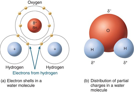
Fig. 1 Schematic depiction of a water molecule¶

The interaction between two water molecules is described by the sum of a Coulombic term and a dispersive term between the oxygen atom of each molecule only:

\[U = \frac{1}{2} \sum_{i=1}^3 \sum_{j=1}^3 \frac{q_i~q_j}{4\pi \varepsilon_0} + \frac{A}{r^{12}_\mathrm{OO}} - \frac{B}{r^{6}_\mathrm{OO}}\]

where $A = 629.4 \times 10^3~\mathrm{kcal\,Å^{12}/mol}$ and $B = 625.5~\mathrm{kcal\,Å^{6}/mol}$. This model is reasonably accurate despite its computational simplicity for the prediction of properties of liquid water at ambient temperature. On the other hand it is not very accurate in describing liquid-solid transitions of water. For example, you can see in Fig. 2 that even an improved spc model of water (spc/e, right) poorly agrees with the experimental diagram (left): it is not able to predict some of the ice phases at all, and the liquid/ice-I (the ice we know) transition is shifted towards lower temperatures.

Fig. 2 Phase diagram of water as obtained from the experiment (left) and from the spc/e model (right). Note the shift of $0.1\,\mathrm{GPa}$ on the y-axis. Adapted from this.¶

Anyway, let us start working on this system.

Setting up your account on Balena¶

Note

This is a one-off setup step that you have to do as this is your first time on Balena. You will never have to do it again.

Start by logging in on the cluster if you are not on it already: you can proceed the same way as you did earlier with linux.bath.ac.uk but this time you need to connect to balena.bath.ac.uk.

You first need to setup your account once for all:

$ cp /beegfs/scratch/group/ce-molsim/brc ~/.bashrc
$ source ~/.bashrc

The best is to copy and paste those lines: ~/.bashrc needs to be typed exactly as it is, with the tilde (~), slash (/) and dot (.) followed by bashrc, without spaces. Once this is done, you are ready to go.

Scratch space¶

Among the files and folders that might already exists in you home directory, you should find one folder named scratch.

That scratch folder is a very special storage space: it is backed by a big array of fast hard-drives. This is where you should do all your calculations, without exception.

Contrary to your home directory, your scratch space is not backed up in principle.

Preparing the simulation¶

Download the required files from this link: water.tar.xz on your local computer.

Copy it over to your home folder on Balena using one of the methods presented in Accessing remote files.

Create folders as you see fit within your scratch space to contain all the files related to this water simulation (e.g. ~/scratch/tutorials/gromacs). Then move (mv) water.tar.xz to that folder, change directories (cd) to reach the file and uncompress the archive:

$ tar xf water.tar.xz

Have a look at the uncompressed files. The most important one is called grompp.mdp as it contains key parameters for running the molecular dynamics simulation. Have a look at it using less. The most important parameters for now are shown in List. 1. These parameters specify that the type of simulation we perform is molecular dynamics using the velocity verlet algorithm (integrator = md-vv), that the time step is dt = 0.002 ps and that we will run the simulation for nsteps = 50000 time steps.

List. 1 water/grompp.mpd¶

; RUN CONTROL PARAMETERS
integrator               = md-vv
; Start time and timestep in ps
tinit                    = 0
dt                       = 0.002
nsteps                   = 50000

The simulation is here performed at a constant temperature of ref_t = 300 K and constant pressure of ref_p = 1.0 bar as shown in List. 2.

List. 2 water/grompp.mpd¶

; Time constant (ps) and reference temperature (K)
tau_t                    = 0.1
ref_t                    = 300
; Time constant (ps), compressibility (1/bar) and reference P (bar)
tau_p                    = 0.5
compressibility          = 4.5e-5
ref_p                    = 1.0

Note

Lines starting with ; in that files are so-called comments or commented lines: they are lines that are completely ignored by Gromacs; they are used to convey human-readable information; in these examples they are used to express what each variable is about and in what units.

Another interesting file is conf.gro that describes the initial configuration of 216 water molecules: you can visualise it either by using Vmd as described in the command line primer tutorial or by installing a suitable program (such as Vmd or CrystalMaker) on your own computer.

Running the simulation¶

Running a simulation on Balena is a convoluted process. You may have a quick glance at How do you submit a job? to get the general idea but you are not expected to understand all these intricacies by yourself: we are going to get there little by little, a step at a time.

For now, the single thing you need to understand is that running simulations on Balena, directly in the command line, is strictly forbidden. When you are on Balena, you log onto the front node. This is used for general accessing of files and folders, but not anything which requires great computing power. We are going to instead, log onto a computing node using a built-in command:

$ sint

If logging on the node was successful, you should see a green computing appear on the prompt. To make Gromacs available to you, you need to load it:

$ module load gromacs/2019.2

A new command, gmx should now be available. This command is used to run Gromacs on the cluster.

Now you are finally all set up to run calculations. First you need to have Gromacs pre-process the input files:

$ gmx grompp -v

This is something you need to do every time you change anything in your input files (for instance if you change the pressure or the temperature of the simulation). Once that pre-processing is finished (hopefully without errors), it is time to start the actual molecular dynamics simulation:

$ gmx mdrun -nt 4 -v

Obviously, both these commands needs to be used in the directory where you placed your input files.

Visualising the dynamics with Vmd¶

You can also use Vmd to visualize individual configurations of the system as well as the complete run. For this follow these steps:

Copy the file spc216.pdb (which contains the initial configuration) and the file traj_comp.xtc somewhere on your computer.
Access linux.bath.ac.uk and start Vmd.
One of the windows that will open will be called VMD Main. Drag and drop the spc216.pdb file into the grey area of the window. This should load the initial configuration of 216 water molecules.
Play around with this configuration using various visualization options from the VMD Main window.
In the VMD Main window click on the line in the main grey area specifying the loaded 216 water molecule configuration. Click File ‣ Load data into Molecule and drop traj_comp.xtc into the new window.

This should create a movie-like visualization of the performed molecular dynamics simulation. Play with it (i.e. move back and forward along time axis, rotate the system, zoom. change colours, etc.).

Analysing the data¶

Now is the time to analyse the results we obtained from the previous simulation. We could start by analysing the trajectory file (traj_comp.xtc) which contains the positions of water molecules at each step of the calculation.

Gromacs provides a post-processing command dedicated to generating various data about hydrogen bonds in the system. In particular, it will give you the average number of hydrogen bonds per molecule of water:

$ gmx hbond -f traj_comp.xtc -xvg none

Select the group you are interested in and plot the resulting number of hydrogen bonds using gnuplot (hbnum.xvg):

$ gnuplot -p -e 'plot "hbnum.xvg" with lines'

It is also possible to calculate the self-diffusion coefficient of water:

$ gmx msd -f traj_comp.xtc -xvg none

Again, choose the group you are interested in and plot the result.

Finally, energy analysis is also possible:

$ gmx energy -f ener.edr -xvg none

In contrast to the other three commands, the energy program analyses the energy file. It will offer you a choice of different properties such as density, potential energy, etc. It reports the average of this characteristic over the simulation time but also saves it in a file (energy.xvg) as a function of simulation time. Regardless of the chosen property, the generated file is always the same energy.xvg. So if you want to keep different output files make sure that you rename the file or it will be overwritten! Units should be reported in the output.

Hint

Excel is also an excellent tool to plot the the content of those files. You can remove the -xvg none flag from the above commands to get a more verbose and detailed version of the output. This detailed output cannot be plotted with gnuplot.

Investigating water properties¶

Now that you have run your first molecular dynamics simulations and processed the data, it’s time now to put these skills into practice. The force field we are using can represent the phase diagram of water fairly well but has its limits —let’s test its boundaries! We can do this by running simulations at different temperatures, from $300\,\mathrm{K}$ to $140\,\mathrm{K}$ in $40\,\mathrm{K}$ steps and by following the thermodynamic properties of each simulation, we can work out at what temperature the force field predicts the phase transition from water to ice occurs. Follow these steps to test it out!

Go up a level in your file hierarchy and make a sub folder for each simulation temperature e.g.
```
$ cp -r water water_300K
```
Go into each directory to change the temperature accordingly in grompp.mpd (ref_t variable, see List. 2)
Perform the simulations in each sub folder, as you did the first time around, by changing into the desired directory and using the two commands for executing Gromacs molecular dynamics simulations:
```
$ gmx grompp -v
$ gmx mdrun -v
```
Use the data analysis tools to watch how the properties of water change with temperature.
Plot the average self-diffusion coefficient against temperature.
Plot the number of hydrogen bonds against temperature.
View your trajectories for each temperature in Vmd.

Hint

Again, using Excel to plot things is fine.

Questions¶

The bulk thermodynamic properties of water at 300 K are:
- Density of water: $997\,\mathrm{kg/m}^3$.
- Diffusion coefficient: $2.4\times10^{-9}\,\mathrm{m}^2\mathrm{/s}$.
Compare your results from your simulation at $300\,\mathrm{K}$ with the experimental properties of water. How different are they?
By analysing your variable temperature water molecular dynamics study, can you work out at which temperature water turns from liquid to ice?
What key parameters change? (Density, hydrogen bonds, diffusion coefficient, etc.)
Do you think spc is a good model for water?