2 Walks
2.1 Generating walks
A walk of length \(L\) from vertex \(i\) to vertex \(j\) in \(G\) is an ordered list of edges of \(G\), \[W = e_1, e_2, \ldots , e_L\] such that \(e_{\ell} = v_{\ell} v_{\ell+1}\) where \(v_1=i\) and \(v_{L+1}=j\).
Informally we write \(W : i \to j\).

\[\begin{aligned} && v_1=B, \quad v_2=A\\ && v_3 = C, \quad v_4=D\end{aligned}\]
\(W = BA, AC, CD\) is a walk of length \(3\) from \(B\) to \(D\).
Proof. Induction on \(L\). For the base case, there is exactly one walk of length one from \(i\) to \(j\) if and only if \(i \sim j\), if and only if \(A_{ij}=1\).
Now suppose true for \(L-1\), we compute \[\begin{aligned} &\text{(number of walks of length $L$ from $i$ to $j$)}\\ &\qquad= \sum_{k \sim i} \text{(number of walks of length $L-1$ from $k$ to $j$)}\\ &\qquad= \sum_{k \sim i} [A^{L-1}]_{kj}\\ &\qquad= \sum_{k} A_{ik}[A^{L-1}]_{kj}\\ &\qquad= [A A^{L-1}]_{ij}\\ &\qquad= [A^{L}]_{ij}. \end{aligned}\]
The walk generating function of a graph (or multigraph or digraph) \(G\) is a matrix-valued function encoding walks of all lengths, it is defined by the formal power series \[\varphi(x) = \sum_{\ell=0}^{\infty} x^{\ell} A^{\ell}.\]
Proof. Write \(\Lambda\) and \(U\) for the eigenvalue and eigenvector matrices of \(A\). First, note that by Theorem 1.8, \[\begin{aligned} A^{\ell} &= (U \Lambda U^T)^{\ell} \\ &= U \Lambda \underbrace{U^T U}_{I} \Lambda \underbrace{U^T U}_{I} \Lambda \ldots \Lambda U^T \\ &= U \Lambda^{\ell} U^T \end{aligned}\] and \[x < \dfrac{1}{\lambda_1} \quad \Rightarrow \quad x\lambda_i < 1 \quad \forall i,\] so \[\sum_{\ell=0}^{\infty} (x \lambda_i)^{\ell} = \dfrac{1}{1-x\lambda_i}\] is a geometric series.
Then we compute \[\begin{aligned} \varphi(x) &= \sum_{\ell=0}^{\infty} x^{\ell} A^{\ell}\\ &= \sum_{\ell=0}^{\infty} x^{\ell} U \Lambda^{\ell} U^T\\ &= U \begin{pmatrix} \ddots &&\\ &\sum_{\ell=0}^{\infty} x^{\ell} \lambda_i^{\ell}&\\ && \ddots \end{pmatrix} U^T\\ &= U \begin{pmatrix} \ddots &&\\ &\dfrac{1}{1-x\lambda_i}&\\ && \ddots \end{pmatrix} U^T\\ &= U (I-x\Lambda)^{-1} U^T \\ &= (U(I-x\Lambda) U^T)^{-1}\\ &= (I-xA)^{-1}. \end{aligned}\]
Proof. \[\begin{aligned} \dfrac{\partial \varphi}{\partial x} &= \sum_{\ell=1}^{\infty} \ell x^{\ell-1} A^{\ell} \\ \dfrac{\partial^2 \varphi}{\partial x^2} &= \sum_{\ell=2}^{\infty} \ell(\ell-1) x^{\ell-2} A^{\ell} \\ \dfrac{\partial^L \varphi}{\partial x^L} &= \sum_{\ell=L}^{\infty} \ell(\ell-1)\ldots(\ell-L+1) x^{\ell-L} A^{\ell} \\ \Rightarrow \dfrac{\partial^L \varphi}{\partial x^L} \Big|_{x=0} &= (L(L-1)\ldots 1) A^L = L! A^L. \end{aligned}\]
Consider an \(n\)-star graph with one vertex of degree \(n\) connected to \(n\) vertices of degree 1. For example, this is a 12-star:

What is the generating function of walks starting and ending at the central vertex?
\[A=\left(\begin{array}{cccc}0&1&1&\dots\\1&0&0&\\1&0&0&\\\vdots&&&\ddots\end{array}\right)\]
\[\det(I-xA)=\left|\begin{array}{cccc}1&-x&-x&\dots\\-x&1&0&\\-x&0&1&\\\vdots&&&\ddots\end{array}\right|=1-nx^2\]
\[\varphi(x)_{1,1}=\big[(I-xA)^{-1}\big]_{11}=\frac{1}{\det(I-xA)}=\frac{1}{1-nx^2}\]
Alternatively, write \(W_L\) for the number of walks of length \(L\) that start and end at vertex 1. Clearly \(W_0=1\) (the empty walk that goes nowhere), and for \(\ell\geq0\) we have \(W_{2\ell+1}=0\) (walks returning to the centre should have even length) and \(W_{2\ell}=n^\ell\) (you have \(n\) choices of which vertex to visit before returning to the centre, for each of \(\ell\) excursions). So
\[\varphi(x)_{1,1}=\sum_{\ell=0}^\infty W_{2\ell}x^{2\ell}= \sum_{\ell=0}^\infty (nx^2)^{\ell}=\frac{1}{1-nx^2}\]
2.2 Centrality
Katz centrality
Who is the most “important” individual in a social network? Sociologist Leo Katz thought status is partly intrinsic and partly earned through relationships. He suggested the measure \[\kappa_i = \underbrace{\alpha \sum_j A_{ij} \kappa_j}_{\text{earned}} + \underbrace{1}_{\text{intrinsic}}\] where \(\alpha\) is a parameter.
Solving this equation gives the following definition. The Katz centrality of vertex \(i\) is the \(i\)-th entry of the vector \(\boldsymbol{\kappa}\) given by \[\begin{aligned} && \boldsymbol{\kappa}= \alpha A \boldsymbol{\kappa}+ \boldsymbol{1} \\ && \boldsymbol{\kappa}= (I-\alpha A)^{-1} \boldsymbol{1} = \varphi(\alpha) \boldsymbol{1} \end{aligned}\] where \(\alpha\) is a tunable parameter.
Consider the star graph again with \(n\) vertices attached to a single central vertex. The outer vertices \(2,\ldots,n+1\) are all identical, so \(\kappa_i=\kappa_2\) for \(i=3,\ldots,n\). We therefore have to solve
\[\kappa_1=\alpha n\kappa_2+1, \quad \kappa_2=\alpha\kappa_1+1\]
The solution is
\[ \kappa_1=\frac{1+n\alpha}{1-n\alpha^2}\,,\quad \kappa_2=\frac{1+\alpha}{1-n\alpha^2}\]
So the central vertex has a higher score than the outer vertices. For example, if \(n=10\) and \(\alpha=0.2\) then \(\kappa_1=5,\,\kappa_2=2\).
Proposition 2.4 The parameter \(\alpha\) interpolates Katz centrality between
\(\kappa_i \approx 1 + \alpha d(i)\) when \(\alpha \ll 1\)
\(\boldsymbol{\kappa}\approx \dfrac{1}{1-\alpha \lambda_1} \boldsymbol{v}_1 \|\boldsymbol{v}_1\|_1\) when \(\alpha \approx \dfrac{1}{\lambda_1}\).
Proof. For (i) we will prove \[\lim_{\alpha\to 0} \dfrac{\kappa_i-1}{\alpha} = d_i.\] From Proposition 2.2 we have \[\begin{aligned} \kappa_i &= \sum_j \varphi_{ij}(\alpha)\\ &= \sum_{L=0}^{\infty} \alpha^L \sum_j [A^L]_{ij}\\ &= 1 + \alpha \underbrace{\sum_j A_{ij}}_{d(i)} + \underbrace{\sum_{L \geq 2} \alpha^L \sum_j [A^L]_{ij}}_{O(\alpha^2)} \end{aligned}\] Thus \[\dfrac{\kappa_i-1}{\alpha} = d(i) + O(\alpha) \to d(i) \quad \text{as $\alpha \to 0$}.\]
For (ii) we will prove \[\lim_{\alpha \nearrow \frac{1}{\lambda_1}} \boldsymbol{\kappa}(1-\alpha \lambda_1) = \boldsymbol{v}_1 \|\boldsymbol{v}_1\|_1.\] Write \(U=(\boldsymbol{v}_1 \ldots \boldsymbol{v}_n)\) for the orthonormal matrix of eigenvectors of \(A\), from Proposition 1.8. So \[A = U \Lambda U^T\] with \[\Lambda = \text{diag} (\lambda_1 \ldots \lambda_n).\] Then \[\begin{aligned} \boldsymbol{\kappa}(1-\alpha \lambda_1) &= (1-\alpha\lambda_1)(I-\alpha A)^{-1} \boldsymbol{1}\\ &= (1-\alpha\lambda_1) U (I-\alpha \Lambda)^{-1} U^T \boldsymbol{1}\\ &= U \begin{pmatrix} 1 &&& \\ & \ddots &&\\ && \dfrac{1-\alpha \lambda_1}{1-\alpha \lambda_i} &\\ &&& \ddots \end{pmatrix} U^T \boldsymbol{1} \quad \text{as $\alpha \nearrow \frac{1}{\lambda_1}$}\\ &\to U \begin{pmatrix} 1 &&& \\ & 0 &&\\ && \ddots &\\ &&& 0 \end{pmatrix} U^T \boldsymbol{1}\\ &= (\boldsymbol{v}_1 \ldots \boldsymbol{v}_n) \begin{pmatrix} 1 &&& \\ & 0 &&\\ && \ddots &\\ &&& 0 \end{pmatrix} \begin{pmatrix} \boldsymbol{v}_1^T \\ \vdots\\ \boldsymbol{v}_n^T \end{pmatrix} \begin{pmatrix} 1 \\ 1\\ \vdots\\ 1 \end{pmatrix}\\ &= (\boldsymbol{v}_1 \ldots \boldsymbol{v}_n) \begin{pmatrix} \boldsymbol{v}_1^T \\ 0\\ \vdots\\ 0 \end{pmatrix} \begin{pmatrix} 1 \\ 1\\ \vdots\\ 1 \end{pmatrix}\\ &= \boldsymbol{v}_1 \|\boldsymbol{v}_1\|_1.\end{aligned}\]
Pagerank
Google use a variation of Katz centrality to rank search results. Katz biases towards high degree vertices and their immediate neighbours (e.g., wikipedia citations). To avoid this, Larry Page proposed \[\pi_i = \alpha \sum_{j} A_{ij} \dfrac{\pi_j}{d{(j)}} + 1.\]
Defining \[D = \begin{pmatrix} d(1) &&0\\ & \ddots & \\ 0 && d(n) \end{pmatrix}\] to be the diagonal matrix of vertex degrees, we can rewrite the above \[\begin{aligned} && \boldsymbol{\pi} = \alpha A D^{-1} \boldsymbol{\pi} + \boldsymbol{1}\\ &\Rightarrow& (I - \alpha A D^{-1} ) \boldsymbol{\pi} = \boldsymbol{1}\\ &\Rightarrow& \boldsymbol{\pi} = D (D - \alpha A)^{-1} \boldsymbol{1}\end{aligned}\]
This is the definition of the pagerank vector \(\boldsymbol{\pi}\). Google uses \(\alpha=0.85\).
2.3 Contagion
Non-backtracking walks
A non-bactracking walk in \(G\) is a walk \(W = e_1, \ldots, e_L\) such that \[e_{\ell+1} \neq e_{\ell} \quad \forall \ell=1,\ldots, L-1.\]
The Hashimoto (or non-backtracking) matrix \(H\) of a graph \(G\) is the \(2|E| \times 2|E|\) matrix with rows and columns indexed by directed edges \(e=i \to j\) and entries \[H_{i \to j, k \to \ell} = \begin{cases} 1 & \text{if $k=j$ and $\ell \neq i$}\\ 0 & \text{else}. \end{cases}\]
Note that \([H^L]_{i \to j, k \to \ell}\) gives the number of non-backtracking walks \(W: e_1, \ldots, e_{L+1}\) in \(G\) such that \(e_1 = ij\) and \(e_{L+1}=k \ell\).

The non-zero entries of \(H\) are: \[\begin{aligned} & (1,2) \\ & (2,3) \quad (2,7)\\ & (3,1)\\ & (4,5) \quad (4,7)\\ & (5,6)\\ & (6,4)\\ & (8,3) \quad (8,5)\end{aligned}\]
Contagion process
A contagion process with transmissibility \(T \in [0,1]\) on a graph \(G\) is defined as:
Initially a single vertex is “infected” .
Each newly-infected vertex has one chance to infect each neighbour, happening independently with probability \(T\).
Repeat (2) until no further transmission is possible.
The risk of vertex \(i\) is the probability it gets infected eventually, given that the infection didn’t die out in it’s early stages. If all infections die out in their early stages then the risk is zero.
A close approximation to risk is given by \[r_i = 1 - \prod_{j \sim i} (1-t_{ji}),\] where \(t_{ji}\) is the probability of transmission from \(j\) to \(i\), which in turn satisfies \[t_{ji} = T \left(1 - \prod_{k \sim j, k \neq i} (1-t_{kj}) \right).\]
Note: this rule is exact in some cases and certain limits, but generally it is just a useful approximation.
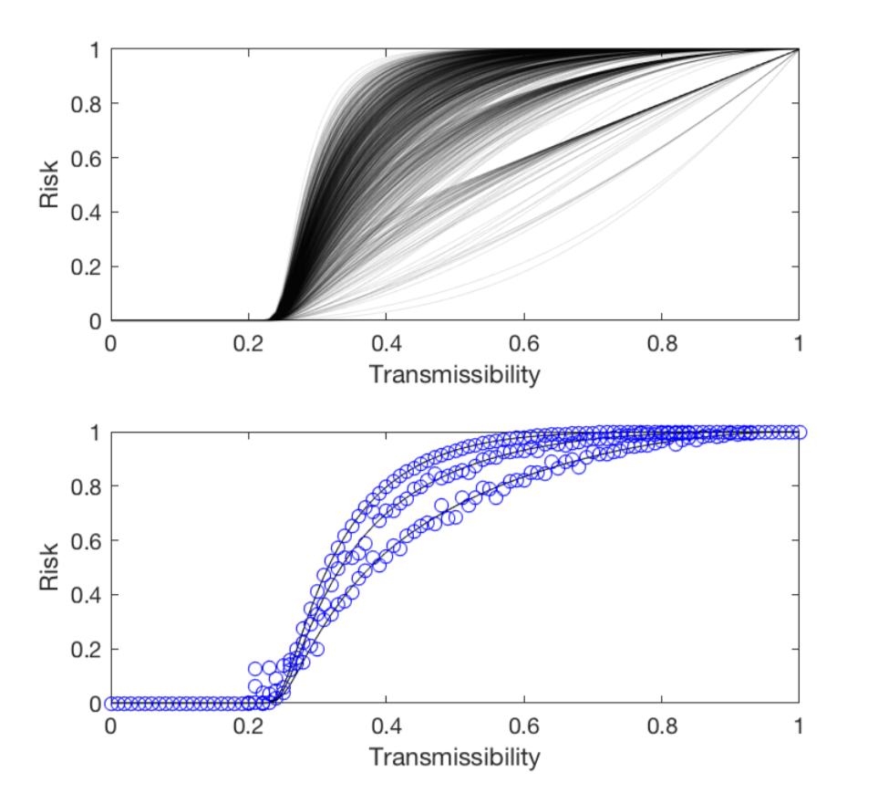
Here is a typical risk profile:

In the top plot, each black line is the risk of one vertex in a randomly generated graph (more on this later). In the bottom plot the black lines are the risk profiles of three different vertices chosen from thr graph; the circles are results of simulations of the contagion process described above.
Note two important features:
there is a critical value of \(T\) below which the risk is zero
the rank ordering of vertex risk changes with \(T\).
Contagion threshold
Proposition 2.5 Define \[T_c := \dfrac{1}{\lambda_{\max}(H)}\] and let \(\boldsymbol{h}\) be the corresponding top eigenvector of the Hashimoto matrix; \[\boldsymbol{h} = T_c H \boldsymbol{h}.\]
Then
If \(T<T_c\) then \(r_i=0 \quad \forall i\).
If \(T=T_c+\varepsilon\) for \(\varepsilon \ll 1\), then \[r_i \propto \varepsilon \sum_{j \sim i} h_{ji}.\]
If \(T=1-\varepsilon\) for \(\varepsilon \ll 1\), then \[r_i \approx 1 - \varepsilon^{d(i)}.\]
Proof. We take the statements in order:
The \(t_{ji}\) obey \(\boldsymbol{t} = F(\boldsymbol{t})\), when \(F : \mathbb{R}^{2|E|} \to \mathbb{R}^{2|E|}\) is defined by \[F_{\ell}(\boldsymbol{t}) = T \left(1 - \prod_{\ell' \stackrel{H}{\to} \ell} (1-t_{\ell'}) \right).\] Note that \(\boldsymbol{t} = \boldsymbol{0}\) is always a solution. We check if it is stable under \(F\) by calculating the Jacobian \[J_{\ell \ell'} = \dfrac{\partial F_{\ell}}{\partial t_{\ell'}} \Big|_{\boldsymbol{t} = \boldsymbol{0}} = T H_{\ell \ell'}.\] If \(T < T_c\) then \[\lambda_{\max} (J) = T \lambda_{\max}(H) < 1,\] so \(\boldsymbol{0}\) is stable and \[r_i = 1 - \prod_{j \sim i} (1-\boldsymbol{0}_{ji}) = 0.\] Otherwise, zero is unstable and another solution must exist.
If \(T=T_c+\varepsilon\) we can guess \(\boldsymbol{t} \approx \varepsilon \boldsymbol{t}'\) for some \(\boldsymbol{t}' \in \mathbb{R}^{2|E|}\). Then \[\begin{aligned} t_{\ell}' &= \dfrac{1}{\varepsilon} t_{\ell} \\ &= \dfrac{1}{\varepsilon} F_{\ell}(\boldsymbol{t}) \\ &= \dfrac{1}{\varepsilon} F_{\ell}(\varepsilon\boldsymbol{t}') \\ &= \dfrac{T}{\varepsilon} \left(1 - \prod_{\ell' \stackrel{H}{\to} \ell} (1-t_{\ell'}) \right) \\ &= \dfrac{T_c+\varepsilon}{\varepsilon} \left(1 - \left[ 1 - \varepsilon \sum_{\ell' \stackrel{H}{\to} \ell} t'_{\ell'} + \ldots \right] \right) \\ &= T_c(H\boldsymbol{t}')_{\ell} + \mathcal{O}(\varepsilon). \end{aligned}\] Thus \(\boldsymbol{t}' \propto \boldsymbol{h}\), and \[\begin{aligned} r_i &= 1 - \prod_{j \sim i} (1- \varepsilon t'_{ji}) \\ &= \varepsilon \sum_{j \sim i} t'_{ji} \\ &\propto \varepsilon \sum_{j \sim i} h_{ji}. \end{aligned}\]
If \(T=1\) then \(\boldsymbol{t}=\boldsymbol{1}\) is a solution. If \(T = 1-\varepsilon\), then we can write a power series for \(\boldsymbol{t}\) \[t_{ji} = 1 - c_{ji} \varepsilon + \ldots,\] where \(c_{ji}>0\) is a constant. But \[\begin{aligned} & t_{ji} = T \left(1 - \prod_{k \sim j, k \neq i} (1-t_{kj}) \right)\\ &\Rightarrow 1 - c_{ji} \varepsilon + \ldots = (1-\varepsilon) - (1-\varepsilon) \prod_{k \sim j, k \neq i} c_{kj} \varepsilon + \ldots \\ &\Rightarrow c_{ji} = 1, \end{aligned}\] so \[r_{i} \approx 1 - \prod_{j \sim i} (1-(1-\varepsilon)) = 1 - \varepsilon^{d(i)}.\]
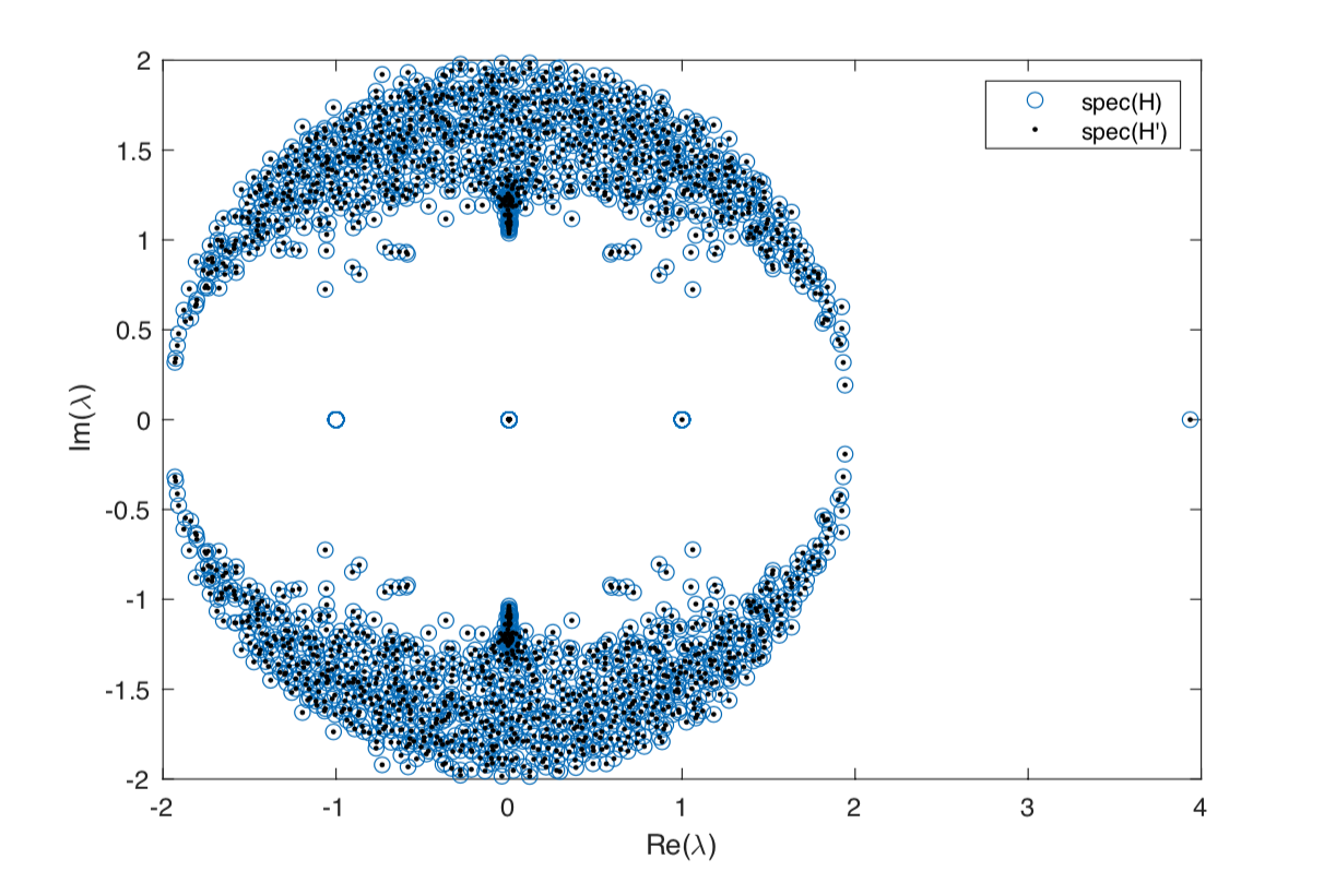
Why is this useful? Well, \(H'\) is generally far smaller than \(H\), so the eigenvalue calculation is quicker.

Here is an Argand diagram showing the eigenvalues of \(H\) and \(H'\) from the above example. Note the top eigenvalue at \(\lambda_{\max}(H)=3.9366\) corresponding to the contagion threshold of \(T_c=0.254\).
2.4 Paths and cycles
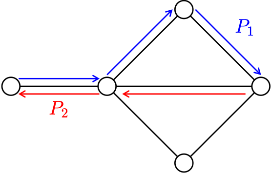
A path is a walk that does not repeat interior vertices. That is if \(P = e_1, e_2, \ldots, e_L\) with \(e_{\ell} = v_{\ell} v_{\ell+1}\), then \(v_i\neq v_j\), \(\forall i \neq j\), except possibly \(v_1=v_{L+1}\).
If \(W_1:u\to x\) and \(W_2:x \to v\) are walks, we write \(W_1 W_2: u \to v\) for the concatenation walk from \(u\) to \(v\). Note that if \(P_1\) and \(P_2\) are paths, \(P_1 P_2\) may not be a path.

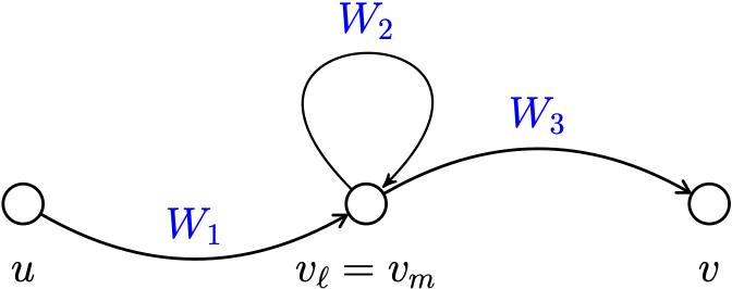
Proof. Let \(W:u \to v\) be a walk. If there is no pair \(\ell < m\) such that \(v_{\ell} = v_m\) is \(W\), then \(W\) is a path and we are done.
If there is such a pair then we may write \[W = W_1 W_2 W_3,\] when \[\begin{aligned} && W_1: u \to v \\ && W_2: v_{\ell} \to v_m = v_{\ell} \\ && W_3: v_{\ell} \to v \end{aligned}\]

Then \(W' = W_1 W_3\) is a walk from \(u\) to \(v\) that contains only edges of \(W\) but is strictly shorter. Repeating this process for all duplicated vertices eventually yeilds a path \(P : u \to v\).
Connectedness
We say \(u, v \in V\) are connected in \(G\) if \(u=v\) or if there is a path \(P:u \to v\). We write \(u \leftrightarrow v\) for short.
Proof. Exercise.
The equivalence classes of \(\leftrightarrow\) are called connected components. Write \(c(G)\) for the number of connected components. If \(c(G)=1\) then we say \(G\) is connected.
Consider the function \(f(n)=n+2\) acting on the ring \(\mathbb{Z}/n\mathbb{Z}\). Let \(G_n\) be the graph with vertex set \(\{0,\ldots,n-1\}\) and edges \(E=\{\{a,b\}\,:\,a=f(b)\}\).
\(G_n\) is connected if \(n\) is odd; if \(n\) is even then \(c(G_n)=2\) and the connected components are the odd and even numbers.

\(n=12\) vs \(n=11\)
The distance from \(u\) to \(v\) in \(G\) is the length of the shortest path \(P: u \to v\), or \(\infty\) if there is they are not connected.
The diameter of a graph \(\text{diam}(G)\) is the maximum distance between vertices.
Let \(G\) be the \(n\)-dimensional hypercube. Vertices are binary strings of length \(n\), and there are edges between every pair of strings that different in only one bit, e.g. \[(0,1,1,0,1)\begin{cases}(1,1,1,0,1)\\(0,0,1,0,1)\\(0,1,0,0,1)\\(0,1,1,1,1)\\(0,1,1,0,0)\end{cases}\]
Distance in this graph is given by the number of bits in which the two strings are different (known as the Hamming distance). The diameter is just \(\text{diam}(G)=n\), since the distance from \((0,\ldots,0)\) to \((1,\ldots,1)\) is \(n\), and no two strings can be different in more than \(n\) places.
Cycles
A cycle is a path that starts and ends at the same vertex.
The circumference \(\text{circ}(G)\) is the length of the longest cycle in \(G\), and the girth is the length of the shortest.

\(\text{circ}(G)=16\), \(g(G)=4\)
Triangles and clustering
A cycle of length \(3\) is called a triangle. The local clustering coefficient \(C(v)\) of a vertex \(v\) is defined as \[\begin{aligned} C(v) &= \dfrac{\text{number of triangles containing $v$}}{\text{number of pairs of neighbours of $v$}}\\ &= \dfrac{\text{number of triangles containing $v$}}{\text{number of triangles containing $v$} + \text{number of non-triangles with middle $v$}}\end{aligned}\]
(If \(d(v)<2\) we say \(C(v) = 0\).)
The mean clustering coefficient is \[C(G) = \dfrac{1}{|V| } \sum_{v \in V} C(v).\]

One has clustering coefficient zero, one has clustering coefficient 1/2.
Proof. \[[A^3]_{ii} = \sum_{k,j} A_{ij} A_{jk} A_{ki},\] so if \((i,u,v)\) form a triangle in \(G\), then it is counted twice in the sum: once when \(j=u, k=v\) and once when \(j=v,k=u\).
So \[(\text{number of triangles containing $i$}) = \dfrac12 [A^3]_{ii}.\]
Finally, \[\begin{aligned} (\text{number of pairs of neighbours of $i$}) = \binom{d(i)}{2} = \dfrac{d(i) (d(i) - 1)}{2}. \end{aligned}\]