1 Introduction

1.1 Graphs

A graph (or simple graph) is a pair \(G=(V,E)\) of sets such that each \(e \in E\) is a two-element subset of \(V\).

Elements of \(V\) are called vertices (or nodes); elements of \(E\) are called edges.

\[\begin{aligned} V&=\{1,2,3,4\}\\ E&=\{ \{1,2\} , \{2,3\} , \{2,4\}, \{3,4\} \}\end{aligned}\]

Remember sets ‘ignore’ order and multiplicity, so in a simple graph:

• Edges do not have a direction: \(\{u,v\} = \{v,u\}\).

• Edges have distinct endpoints \(u\neq v\).

• Edges are unique: \(\{\{u,v\},\{u,v\}\} = \{\{u,v\}\}\).

It is common to write \(uv\) as a shorthand for the edge \(\{u,v\}\), when there is no chance of confusion.

Multigraphs and digraphs

A multigraph allows multiple edges and loops. A directed graph or digraph has directed edges \((u,v)\in V^2 \supset E\).

A multigraph:

A digraph:

Unless stated otherwise, the graphs in this unit are all simple graphs.

Empty graphs and complete graphs

For fixed \(V\): the empty graph has no edges, so \(E=\emptyset\); the complete graph has every possible edge, so \[E = \{ \{u,v\} : u,v \in V, u \neq v \}.\]

The complete graph on \(n\) vertices is referred to by the notation \(K_n\).

Graph isomorphism

Two graphs \(G=(V,E)\) and \(G'=(V',E')\) are isomorphic if there exists a bijection \(f:V \to V'\) such that \[\{u,v\} \in E \quad \Leftrightarrow \quad \{f(u),f(v)\} \in E'.\]

We write \(G \simeq G'\) if this is the case.

\(u\)	\(1\)	\(2\)	\(3\)	\(4\)	\(5\)
\(f(u)\)	\(\mathrm{ii}\)	\(\mathrm{iii}\)	\(\mathrm{v}\)	\(\mathrm{iv}\)	\(\mathrm{i}\)

Note \(f\) is not unique in this case.

Here is a more interesting example of graph automorphism. The “Möbius ladder” is isomorphic to a “wheel” with an even number of spokes:

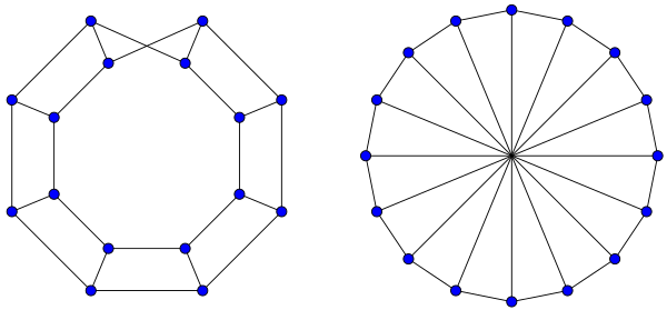
It can be very difficult to determine if two graphs are isomorphic to each other, and there is no general formula for the number of isomorphism classes of graphs of a given size.

\(|V|\)	\(1\)	\(2\)	\(3\)	\(4\)	\(5\)	\(6\)	\(\ldots\)	\(n\)
#graphs	\(1\)	\(2\)	\(8\)	\(64\)	\(1024\)	\(32768\)	\(\ldots\)	\(2^{\binom{n}{2}}\)
#isomorphism classes	\(1\)	\(2\)	\(4\)	\(11\)	\(34\)	\(156\)	\(\ldots\)	??

Subgraphs, neighbourhoods and degrees

• A subgraph \(G' \subseteq G =(V,E)\) is a graph \(G'=(V',E')\) such that \(V' \subseteq V\) and \(E' \subseteq E\).

• An induced subgraph of \(G=(V,E)\) is a subgraph of the form \(G'=(V',\{uv\in E\,|\,u,v\in V'\})\). That is, it includes all possible edges from the original graph for a given subset of vertices.

• Vertices \(u,v \in V\) are adjacent (or neighbouring) in \(G\) if \(uv \in E\). We may write \(u \sim v\) or \(u \sim_G v\). The neighbourhood \(\mathcal{N}(v) = \mathcal{N}_G(v)\) is the set of all neighbours.

• The degree \(d(v) = d_G(v)\) of a vertex is the size of its neighbourhood, i.e. \[d(v) = |\mathcal{N}(v)| = |\{u \in V : uv \in E\}|.\]

• The average degree of a graph is \[d(G) = \dfrac{1}{|V|} \sum_{v \in V} d(v).\]

• The maximum and minimum degrees are \[\Delta(G) = \max_{v \in V} d(v)\,,\quad \delta(G) = \min_{v \in V} d(v)\,.\]

\[\begin{aligned} & d(1)=1,\quad d(2)=4,\quad d(3)=3\\ & d(4)=3,\quad d(5)=3,\quad d(6)=0\\ & \delta(G) = d(6) = 0\\ & \Delta(G) = d(2) = 4\\ & d(G) = 7/3\end{aligned}\]

\[G'=(\{2,3,4\},\{\{2,3\},\{3,4\}\})\subseteq G\]

Proposition 1.1 (The Handshaking Lemma) For every simple graph \(G\), \[\sum_{v \in V} d(v) = 2|E|\,.\]

Proof. Every edge has exactly two endpoints, so when summing degrees we count each edge twice.

Notice the narrative style of proof - this is common in graph theory. The theorems often involve counting or classifying things in two different ways, hence the job of the proof is to convince the reader that both methods are correct. Occasionally, however, a simple calculation is possible…

Proposition 1.2 \[d(G) = \dfrac{2|E|}{|V|}.\]

Proof. \[\begin{aligned} d(G) &= \dfrac{1}{|V|} \sum_{v \in V} d(v)\quad \text{(by definition)}\\ &= \dfrac{1}{|V|} 2|E| \quad \text{(by handshaking)} \end{aligned}\] \(\quad\)

Proposition 1.3 Every graph has an even number of vertices of odd degree.

Proof. Exercise.

1.2 Graphical sequences

The degree sequence of a graph \(G\) is the list \[\boldsymbol{d}(G) = (d_1, \ldots, d_{|V|})\] of degrees of vertices in \(G\), written in descending order \[d_1 \geq d_2 \geq \ldots \geq d_{|V|}.\]

Note that \(d_1 = \Delta(G)\) and \(d_{|V|}=\delta (G)\).

An arbitrary sequence \(\boldsymbol{d} \in \mathbb{N}^n\) is said to be graphical if there exists a graph \(G\) for which \(\boldsymbol{d}\) is the degree sequence.

Proposition 1.4 (Erdős-Gallai) A sequence \(d_1 \geq \ldots \geq d_n\) is graphical if and only if \(\sum_i d_i\) is even and for all \(k \in \{1,\ldots,n\}\) we have \[\sum_{i=1}^k d_i \leq k(k-1) + \sum_{i=k+1}^n \min \{d_i,k\}\]

Proof. (\(\Rightarrow\)) Exercise (\(\Leftarrow\)) Too hard. See Erdős, Gallai (1960) if you can read Hungarian, or Tripathi, Sushmita, West (2010) if you can’t.

Suppose \(\boldsymbol{d}=(9,9,8,8,8,8,8,8,2,2)\). Let’s test \(k=3\) (this is the first \(k\) for which \(\min\{d_i,k\}\) isn’t always just \(k\)). In this case we have \[\sum_{i=1}^kd_i=d_1+d_2+d_2=26\] but \[\begin{aligned} k(k-1)&+\sum_{i=k+1}^n\min\{d_i,k\} \\&=3(3-1)+5\times\min\{8,3\}+2\times \min\{2,3\} = 25, \end{aligned}\] so the sequence is not graphical.

Proposition 1.5 (Havel-Hakimi) A sequence \(d_1 \geq \ldots \geq d_n\) is graphical if and only if \[\boldsymbol{d}' = (d_2-1, d_3-1, \ldots, d_{d_1+1}-1, d_{d_1+2}, \ldots, d_n)\] is graphical (after re-ordering if needed).

\[\begin{aligned} & \boldsymbol{d}=(4,4,4,3,2,1)\\ & \boldsymbol{d}'=(3,3,2,1,1)\\ & \boldsymbol{d}''=(2,1,0,1) \mapsto (2,1,1,0)\\ & \boldsymbol{d}'''=(0,0,0)\quad \text{empty $\Rightarrow$ graphical} \end{aligned}\]

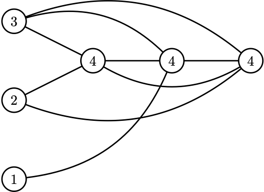
To prove the Havel-Hakimi theorem, we need to think about “rewiring” graphs. Given edges \(uv, xy \in E\) such that \(ux, vy \not\in E\), a two-switch modifies the graph by deleting \(uv\) and \(xy\), then adding \(ux\) and \(vy\).

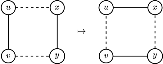
Write \(G \stackrel{2}{\longleftrightarrow} G'\) if \(G\) can be transformed into \(G'\) by a sequence of two-switches (and back by reversing the sequence).

Proposition 1.6 Let \(G\) be a graph on \(V=\{v_1, \ldots,v_n\}\) with degree sequence \(d_1 \geq \ldots \geq d_n\), where \(d_G(v_i)=d_i\).

Then there exists a graph \(H \stackrel{2}{\longleftrightarrow} G\) with \[\mathcal{N}_H (v_1) = \{v_2, \ldots,v_{d_1+1}\}.\]

Proof. Suppose \[\mathcal{N}_G (v_1) \neq \{v_2, \ldots,v_{d_1+1}\},\] then there is an \(i \in \{2,\ldots,d_1+1\}\) such that \(v_i\) is not adjacent to \(v_1\). We look for a two-switch to fix this.

Since \(|\mathcal{N}_G(v_1)|=d_1\), there must be a vertex \(v_j \in \mathcal{N}_G(v_1)\) with \(j > d_1+1\). Also since \(d_i \geq d_j\) (because \(i \leq d_1+1<j\)) and \(v_j \sim v_1\), there must exist another vertex \(v_{\ell}\) that is neighbours with \(v_i\) but not \(v_j\).

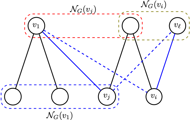
Performing a two-switch on \(v_1 v_j\) and \(v_i v_{\ell}\) gives us a new graph \(G'\) with \(v_i \in \mathcal{N}_{G'}(v_1)\).

Repeating this process for all \(i \in \{2,\ldots,d_1+1\}\) gives \(H\), as required.

Proposition 1.7 (Berge) Two graphs \(G\) and \(H\) with the same vertex set \(V\) satisfies \[d_G(v) = d_H(v)\] for all \(v \in V\) if and only if \(G \stackrel{2}{\longleftrightarrow} H\).

Proof. (\(\Leftarrow\)) Two-switches preserve vertex degrees.

(\(\Rightarrow\)) Induction on \(n=|V|\).

Base case \(n=1\) is trivial.

Suppose the claim holds for graphs of size \(n\) and suppose \(G\) and \(H\) are of size \(n+1\), where \[d_G(v) = d_H(v)\quad \forall v \in V.\]

Label the elements of \(V\) in decreasing order of degree, and apply Proposition 1.6 to obtain graphs \(G' \stackrel{2}{\longleftrightarrow} G\) and \(H' \stackrel{2}{\longleftrightarrow} H\) with \[\mathcal{N}_{G'}(v_1) = \mathcal{N}_{H'}(v_1).\]

Write \(G' - v_1\) for the graph created from \(G'\) by deleting \(v_1\) and similarly for \(H'-v_1\).

These graphs are linked by two-switches by the inductive hypothesis. Applying the same two-switches to \(G'\) obtains \(H'\), so \[G \stackrel{2}{\longleftrightarrow} G' \stackrel{2}{\longleftrightarrow} H' \stackrel{2}{\longleftrightarrow} H.\]

Proposition 1.5 (Havel-Hakimi)
A decreasing sequence \(\boldsymbol{d}\) is graphical iff \[\boldsymbol{d}' = (d_2-1, \ldots, d_{d_1+1}-1, d_{d_1+2}, \ldots,d_n)\] is after re-ordering.

Proof. (\(\Leftarrow\)) Suppose \(\boldsymbol{d}'\) is graphical after re-ordering and \(G'=(V',E')\) is a graph with that degree sequence and vertices labelled \(v_2, \ldots, v_n\).

Construct \(G\) by adding a vertex \(v_1\) and connecting it to each of \(v_2, \ldots, v_{d_1+1}\).

Then \(G\) is a graph with degree sequence \(\boldsymbol{d}\).

(\(\Rightarrow\)) Suppose \(\boldsymbol{d}\) is graphical and \(G\) is a graph with vertices \(v_1 \ldots v_n\) and degrees \(d_G(v_i)=d_i\). Proposition 1.6 gives us \(H \stackrel{2}{\longleftrightarrow} G\) with \[\mathcal{N}_H (v_1) = \{ v_2,\ldots,v_{d_1+1}\}\] and Proposition 1.7 says \(H\) has degree sequence \(\boldsymbol{d}\). Remove \(v_1\) from \(H\) to find a graph \(G'=H-v_1\) with degree sequence \(\boldsymbol{d}'\).

1.3 Adjacency matrices

Let \(G\) be a (simple) graph on the vertices \(V=\{1,\ldots,n\}\). The adjacency matrix of \(G\) is the \(n \times n\) matrix \(A\) with entries \[A_{ij} = \begin{cases} 1 & \text{if $\{i,j\}\in E$}\\ 0 & \text{else} \end{cases}\]

This concept is generalised to directed graphs: \[A_{ij} = \begin{cases} 1 & \text{if $i\to j \in E$}\\ 0 & \text{else} \end{cases} \qquad \text{(note this matrix may not be symmetric)}\] ...and multigraphs: \[A_{ij} = \text{number of edges between $i$ and $j$.}\]

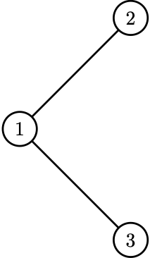\(A = \begin{pmatrix} 0 & 1 & 1 \\ 1 & 0 & 0 \\ 1 & 0 & 0 \end{pmatrix}\)

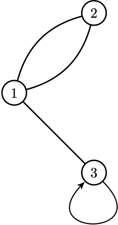\(A = \begin{pmatrix} 0 & 2 & 1 \\ 2 & 0 & 0 \\ 1 & 0 & 1 \end{pmatrix}\)

\(A = \begin{pmatrix} 0 & 1 & 1 \\ 0 & 0 & 0 \\ 1 & 0 & 0 \end{pmatrix}\)

Proposition 1.8 (Perron-Frobenius for adjacency matrices) Let \(A\) be the adjacency matrix of a graph \(G\) with eigenvalues \(\lambda_1\geqslant \ldots\geqslant \lambda_n\), written in order of magnitude, and corresponding eigenvectors \(\boldsymbol{v}_1, \ldots, \boldsymbol{v}_n\). Then

1. \(\lambda_1\geqslant |\lambda_i|\) for all \(i\), and we can choose \(\boldsymbol{v}_1\) with all entries non-negative.

2. For all \(\boldsymbol{w} \in \mathbb{R}^n\) we have \(\lambda_n\sum_iw_i^2\leqslant \sum_{i,j} A_{i,j}w_i w_j \leqslant \lambda_1 \sum_iw_i^2\).

3. \(\delta(G) \leqslant \lambda_1 \leqslant \Delta(G)\).

4. The eigenvectors form a basis of \(\mathbb{R}^n\).

If \(G\) is a multigraph then i-iv all hold. If \(G\) is a digraph then i-iii hold, but not iv, and the eigenvalues and eigenvectors numbered from 2 to \(N\) are complex in general.

Proof. Too long and not relevant for us.

\[A=\left(\begin{array}{cccccccc} &1&1&&1&&&\\ 1&&&1&&1&&\\ 1&&&1&&&1&\\ &1&1&&&&&1\\ 1&&&&&1&1&\\ &1&&&1&&&1\\ &&1&&1&&&1\\ &&&1&&1&1&\\ \end{array}\right)\]

Eigenvalues: \(\{-3,-1,-1,-1,1,1,1,3\}\)

\(\lambda_1=3,\qquad \boldsymbol{v}_1=(1,1,1,1,1,1,1,1)^T\)

Note that in this case \(\delta(G)=\Delta(G)=3\) so from (iii) we know \(\lambda_1=3\) without having to diagonalise \(A\).

Here is a plot of \(\boldsymbol{w}^TA\boldsymbol{w}\) as a function of \(\boldsymbol{w}^T\boldsymbol{w}\) for 10,000 vectors with Guassian random entries (i.e. \(w_i\) is normally distributed). You can see how the bounds in point (ii) above confine the range of values.

Continued Below is the Matlab code to make the plot. The first line may look weird to you… I used de2bi to construct a list of binary sequences expressing the intgers 0 = [0 0 0] through to 7 = [1 1 1]; these are the coordinates of the corners of the cube. The function pdist builds a matrix of all pairwise distances between a collection of coordinate vectors, but it needs to be wrapped with squareform otherwise it only returns the values of ordered paris (i.e. the top right triangle of the matrix). Finally ==1 will return a logical (true/false) matrix saying which pairs of vertices are at distance one, and the wrapper double will map true \(\mapsto\) 1 and false \(\mapsto\) 0. This gives the adjacency matrix of the cube graph.

>> A = double(squareform(pdist(de2bi(0:7)))==1);
>> spy(A);
>> samples=10000; ww=zeros(1,samples); wAw=zeros(1,samples); 
>> for s=1:samples, w=randn(8,1); ww(s)=w'*w; wAw(s)=w'*A*w; end
>> plot(ww,wAw,'.',[0,20],3*[0,20],'k',[0,20],-3*[0,20],'k')