DC-Sweep Analysis Using ORCAD
Introduction
This CAD (computer aided design) session introduces the DC-sweep and parametric sweep capabilities of OrCAD/PSPICE circuit-simulation software. Attempt to finish all the exercises within the set lab period.
To get the most out of the laboratory, it will be necessary for you to recall the simulation procedures by completing a number of simulation exercises following the first detailed run-through of the simulation types.
Circuit simulation is a very quick method of rapidly gaining insight into circuit operation and the dependence of circuit response on component values and other circuit quantities. It is worth practising it to master the simulation procedures and develop an intuitive feel for what is possible, so that future effort goes into designing interesting circuits and analysing simulation results, rather than setting up and executing the simulation. In other words, exercising your creativity on the design becomes the problem, rather than dealing with the simulator.
You will find it helpful to occasionally refer to the CT1 CAD notes to remind yourself about some aspects of basic circuit entry and simulation.
It is a good idea to create directories for each of your CAD labs to keep relevant files together. Create a new directory called CT2 on H: drive for this particular CAD lab if you can. Subsequent labs can be put in sub-directories CT3, CT4, etc. If you are unable to do this, ask a lab supervisor or demonstrator for help. You must now list this directory as the working directory within the OrCAD/Capture program.
DC Analysis
Enter the circuit in Fig.1 into OrCAD/Capture. Remember to edit component designators and values so that they all correspond with those shown in Fig.1, namely, Vs and Rx as well as the values. Select the voltage source from SOURCE library as VSRC; resistor from ANALOG library as R; and Earth symbol using green, earth point from right-side button in SOURCE library as 0. Vout added using Place Net Alias button The output voltage probe will be added later.
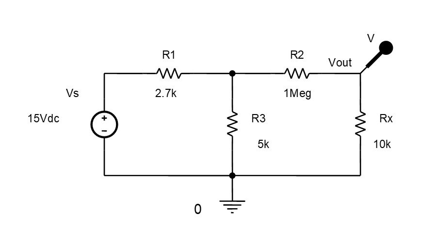
Prepare to run PSPICE to simulate circuit operation by setting up a simulation profile, i.e., from the menu bar select PSpice/New Simulation Profile, set the Name to DC-circuit, and click Create. A Simulation settings dialogue box should open - if you don’t see it, click the flashing last bottom icon - and then close by clicking OK. From the menu bar select PSpice/Run or click on the top encircled arrow Run PSPICE button on the top toolbar.
Add a voltage probe as above using the Voltage/Level Marker button at right of encircled Run PSPICE arrow.
Measure the Vout voltage level given in the results window using the cursor. The cursor is displayed using Trace/Cursor/Display from the result window menu bar, or by pressing the Toggle Cursor button on the top toolbar. Please find the Run and Toggle Cursor buttons now because they will save you time. The voltage level shown in the bottom table should be about 96.271mV. Check your circuit carefully if you do not obtain this value.
DC Sweep
The next analysis investigates how Vout changes as the value of source voltage, VS, is varied (or swept) from 0 to 25V. Some currents in the circuit will also be viewed.
From the Capture menu bar select PSpice/Edit Simulation profile.
In the open dialogue box, set the Analysis type to DC Sweep.
In this example, a linear sweep will be demonstrated. Vout will be plotted while the voltage source VS is swept from 0 V to 25 V in 1 V increments. A linear sweep means that points between the beginning and ending values are equally spaced.
Fill out the dialogue box with the following values:
- Name: Vs
- Start value: 0
- End value: 25
- Increment: 1
Click on Apply and then OK to close the dialogue box. Run PSPICE with the new simulation profile (arrow button). You should obtain the following graph show-ing how VRX varies. Click on bottom flashing icon if the results window does not open automatically.
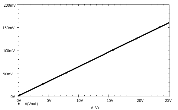
Exercise 1
Use the plot-window cursor from Trace/Cursor/Display to measure $V_{OUT}$ when $V_S$ is 20 V. Note that you will have to position the vertical cursor line approximately using the mouse pointer and a left-button click, and then scroll using the left- and right-pointing cursor keys on the keyboard, until exactly 20.000 is obtained as the X coordinate in the cursor display box. If you cannot get exactly 20.0000, expand the plot-window to full size and try again.
$V_{\text{Out}} \vert _{V_S = 20V}= \qquad V$
You can add as many traces to this graph as you wish. We will now add a second trace. Select Trace and Add Trace from the plot-window toolbar and add I(R1) by clicking on it and clicking OK.
$I(R1)$ is at too low a level to be seen very well on the same vertical scale as VRX. Multiply the $I(R1)$ values by ten. Double click on the $I(R1)$ legend at the bottom of the plot window and change $I(R1)$ to $10 \times I(R1)$. Click OK to close the dialogue box and the variation in $I(R1)$ should now be observable.
Exercise 2
Change a cursor to the current graph and measure the value of I(R1) when VS is 20V.
$I(R1) \vert _{V_S = 20V}= \qquad A$
You may enter quite complicated equations involving any of the plotted quantities. A simple example would be to enter $I(R1) \times I(R1) \times 2.7e3$ to display the the $I^2R$ power loss in R1.
Double click on the $I(R1) \times 10$ legend at the bottom of the plot graph window and enter $I(R1) \times I(R1) \times 2.7e3$ to plot the power. Note that $2.7 \times 10^3$ is input as 2.7e3. Note that the operators and functions that may be used in plot equations are listed on the right-hand side of the dialogue box.
Click OK to display the power in R1. It may be viewed more clearly if you delete the voltage plot by clicking on the V(Vout) legend at the bottom of the plot window and using the keyboard delete to remove that graph.
Exercise 3
Use the plot-window cursor to measure the power dissipated in R1 when VS is 10V. Record the value in your laboratory notebook.
$P_{R1} \vert _{V_S = 10V}= \qquad W$
Delete the voltage marker from your first circuit. Highlight the circuit using a click-hold-sweep-over action and move it out of the way, to the top left-hand corner, for example. Enter the new circuit in Exercise 4, edit the values and edit the simulation profile to generate the required graphs. Note, a quick way to do this is to highlight and copy your old circuit to a free space and then edit it. Otherwise, input the new circuit as before.
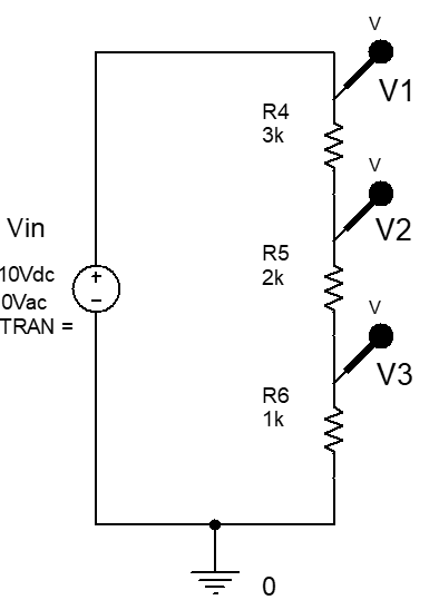
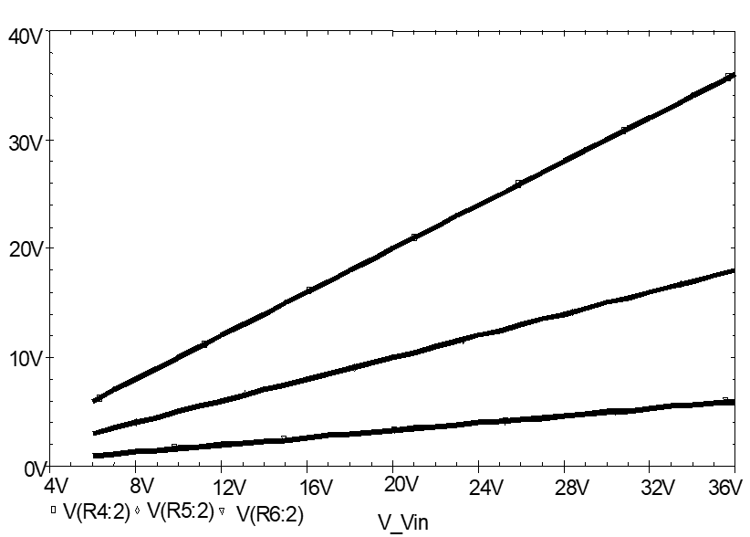
Parametric Sweep
A parametric sweep may be used to analyse the change in a circuit quantity, such as voltage or current, when a circuit parameter other than supply voltage or current, such as a resistance value, is changed.
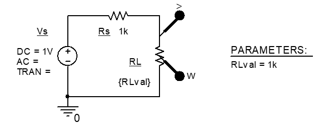
A parametric sweep will now be used to investigate the maximum power a voltage source $V_S$ with an internal resistance of $R_S$ will deliver to a load. In other words, the maximum power theorem, which was derived in CT2 Part 3 of the notes, will be confirmed by varying the value of RL in and monitoring the variation in its power.
Enter the circuit in Fig.3 into OrCAD/Capture. Once again highlight a circuit and drag while pressing Ctrl to copy, and then proceed to editing an old circuit to save time.
You can enter all the circuits for this CAD laboratory on the one worksheet. However, it is a good idea to delete all the voltage and current markers on the circuit you are leaving so that you do not plot results for several circuits together. Also, you will have to be careful not to call voltage sources, resistors, etc by the same name, or reference designator, or the simulation will not run.
From the Options menu select Schematic Page Properties and choose B as your Page Size to accommodate all the circuits coming up.
To vary the value of RL, RL has to be defined as a parameter. Double click on the 1k value of RL and re-place it with the brackets and text {RLval}. Click OK to accept the value.
The value of RL will now be the value of the parameter {RLval}.
Load the SPECIAL library by clicking the Add Library icon. Select Place/Part and from the SPECIAL library, select PARAM and place it adjacent to your circuit.
Double click on the PARAMETERS legend to define the parameter and assign it a default value.
Click on New Property button and enter RLval under Property Name and 1k for Value. Click OK to close.
Click and highlight the new RLval cell that appears in the spreadsheet.
Click on the top toolbar Display button and select Name and Value, so that the name and default value will be displayed with the circuit drawing. Click OK to accept settings.
Close the Properties Editor spreadsheet by clicking the X at window top-centre, below the top row of buttons. Add a voltage V and power W probe as shown.
Your circuit should now resemble , and you can now proceed with a Parameter Sweep simulation.
From the PSpice menu select Edit Simulation profile.
Analysis type should be set at DC Sweep, under Options select Primary Sweep, under Sweep variable select Global parameter, and within Parameter Name enter RLval.
Complete the Sweep type entries as follows:
- Start value: 10
- End value: 100k
- Increment: 100
These Sweep type values give a linear sweep of the value of RLval from $10 \Omega$ to $100 K \Omega$. The selected voltages and currents will be plotted at $100 \Omega$ increments within the specified range, i.e., at 20,000 points.
Click on Apply and OK to select your settings and close the dialogue box.
Selecting the PSpice /Run option, or the green-arrow run-button, should give the result in Fig.5 for the variation in load resistor voltage as the load resistance is increased.
To confirm the maximum power theorem, it is the much smaller values of power in RLval that we require to see. Hence, click V(RL:2) and delete it using the keyboard delete. The rescaled graph should now resemble .
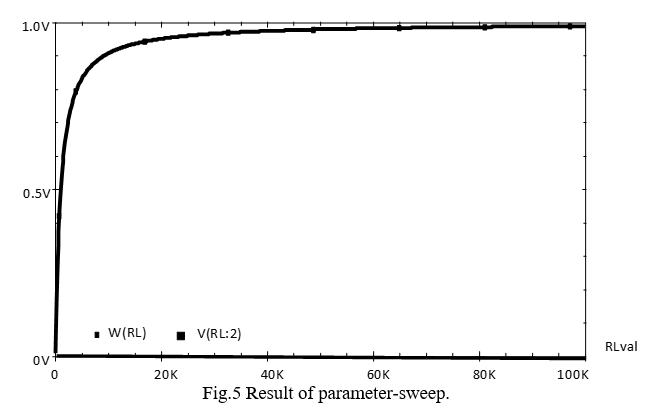
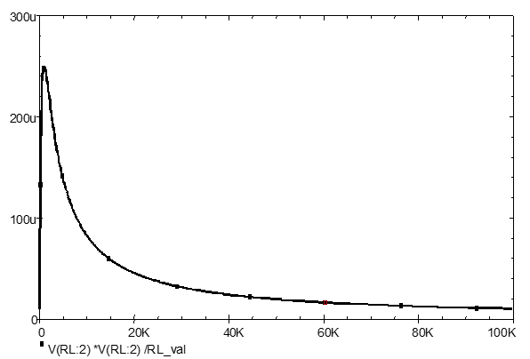
This is not the best way of displaying the power variation since the maximum value occurs at $RLval = 1000\Omega$ and 1000 is quite a small number on the linear axis that has a maximum of 100,000.
Hence, we need to change the X-axis to a logarithmic scale to expand the lower end of the X-axis and com-press the upper end as shown in .
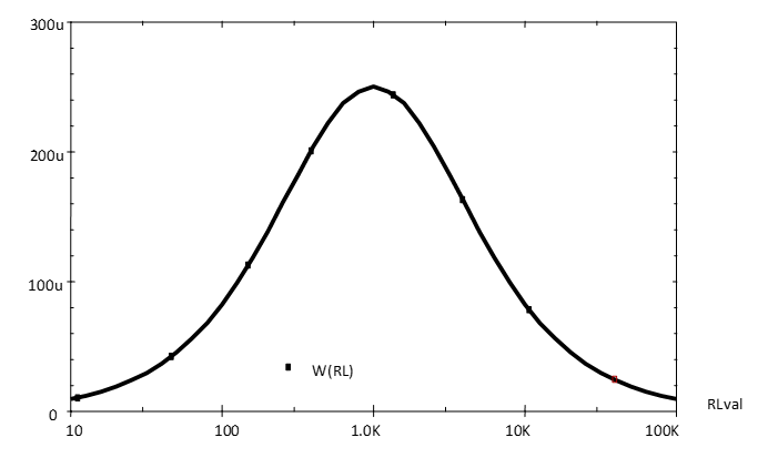
To change the X-axis, within the plot results window, select Plot and then Axis Settings. The current Scale setting should be linear; change the Scale setting to log and click OK to make the change. A graph similar but not identical to with a more easily observed maximum should then be obtained.
Notice that in your logarithmic-axis graph there are not enough points in the first decade (i.e., from 10 to 100) to give a smooth graph even though you have computed 20,000 points. This arises because, with a linear-value sweep plotted on a logarithmic axis, most of the points are crowded towards the right-hand side of the graph. To get an even distribution of points on a log plot, we need to use a logarithmic sweep.
Select Edit Simulation Profile and select Logarithmic Sweep Type, select Decade beside the Logarithmic button now highlighted, and change the Points/decade to 1000.
The range $10 \Omega$ to $100 k \Omega$ extends over 4 decades, and with 1000 points/decade the graph will be made up of only 4000, rather than 20,000 points. However, since the points will be distributed evenly over the log-X axis, all sections of the graph will be plotted with the same resolution. A more useful display of the variation is obtained, and the results take up much less file space.
Exercise 5
Run the simulation again to plot the power variation in the varying load resistor by removing the voltage V probe graph to rescale the power W marker probe results. Observe the smooth lower end of the graph as shown in Fig.7. A log-axis graph should be automatically plotted.
What maximum source power will be delivered when RL is varied from $10\Omega$ to $100 k$? $P_{\text{max}} = \qquad W$
Why does the power go through a maximum with increasing load resistance? Explain why and then check your reasoning by superimposing and making visible current, voltage, and power graphs as explained below.
Add a current probe to the left of RS, run the simulation again. Double click on W(RL) at the graph bottom and multiply by 1000 by changing to W(RL)*1000. In a similar way, multiply the current I(Rs) by 1000.
Exercise 6
Perform a DC sweep simulation using the circuit in Fig.8 to investigate the condition when a practical constant current source with internal resistance, RS1, delivers maximum power to a load resistor RLI. Initially, set up the DC-Sweep to sweep the global parameter RLval logarithmically from $100 \Omega$ to $100 k\Omega$ using 1000 points/decade. Simulate the circuit and, either plot the load resistor power directly using a W marker probe, or plot current using a current I marker and then square this current and multiply by RLval to get a resistor-power plot.
Record:
- the sweep conditions for accurate load-power measurement
- the load resistance for maximum power and use the plot-window cursor keys to determine the
- maximum power value
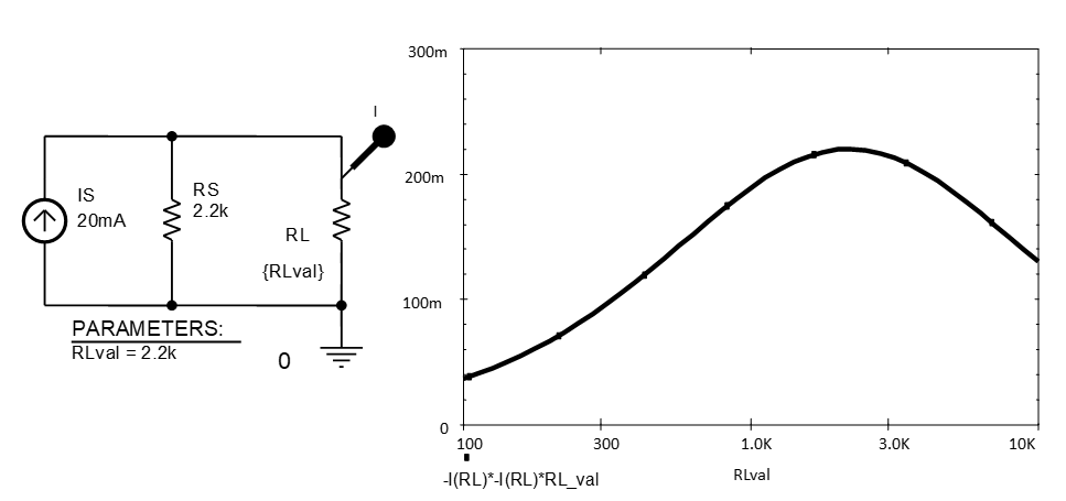
Sweep type, $\qquad$ start $R_L$ value, $\qquad$ stop $R_L$ value, $\qquad$ increment value $\qquad$
$R_L(P_{\text{Max}}) = \qquad \Omega$
$P_{RL{\text{Max}}} = \qquad W$
Exercise 7
Use the previous simulation technique to find the value of load resistor, RL, that allows maximum power to be drawn from the circuit.
Record
- the sweep conditions for accurate load-power measurement
- the load resistance for maximum power and use the plot-window cursor keys to determine the
- maximum power.
If Thevenin’s theorem has been covered before the lab, you can use it to create a Thevenin equivalent circuit, for the part of the circuit to the left of the terminals indicated by circle-symbols, to check your answer.
Sweep type, $\qquad$ start $R_L$ value, $\qquad$ stop $R_L$ value, $\qquad$ increment value $\qquad$
$R_L(P_{\text{Max}}) = \qquad \Omega$
$P_{RL{\text{Max}}} = \qquad W$
Exercise 8
Can you envisage how circuit theory might be useful in understanding or gaining insight into the operation of circuits and how conditions vary as values change, or checking circuit designs before going to the trouble of building and testing? Discuss with an interesting person.
What other components, theorems or design issues could be investigated? Some suggestions are listed below.
Locate the OPAMP part in the ANALOG Part Library. Simulate the op-amp circuit shown below using a Time Domain (Transient) Analysis Type, rather than Bias Pont or DC Sweep, in the Simulation profile to measure input and output voltage. Why is this circuit known as an inverting amplifier?

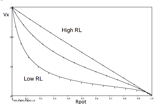
Locate the POT part in the Breakout Part Library. Simulate the effect of a reducing load resistance in a circuit where a potentiometer, i.e., an adjustable voltage divider, is used to vary output voltage. Simulate the circuit using A DC Sweep Analysis Type with Primary Sweep, Global Parameter options checked and set Parameter name: to Rpot and sweep between 0 and 1 with 0.1 step. Note the significant effect on potentiometer linearity of relatively low load resistance, i.e., with $RL \leq 0.1 R_{pot}$, the variation in Vx with pot setting is very nonlinear as above.

Reflection on skills and learning
Complete in your lab notebook outside the lab if you run out of time. Comment on your individual attainment as suggested below.
What percentage of the lab work did you complete? How do you rate your participation as a lab group member?
What level of proficiency do you feel you achieved in entering and simulating circuits and measuring and understanding the DC voltage, current and power value changes with swept supply and component value changes. Choose one of the following and add a comment.
- High –now confident performing DC-sweep and parameter-sweep simulations. Can apply in —-?
- Medium – some further practice required but have reasonable understanding of setting up and running simulations and understand the form of results. More practise in required in —–?
- Basic – can follow the process and results but need greater individual practice to master circuit in-put and interpretation. The main obstacle to more confident application is —–?
List two or more ways in which attending and completing the lab work has been of value.
List any changes to the lab work that you identified which would facilitate circuit theory learning and ac-quiring circuit simulation skills.