Introduction to Instrumentation
Work package IE1 gives experience in using laboratory instrumentation. No previous experience is assumed. All calculations, measurement results, waveform sketches, comments, etc may be written in these notes.
Tutorial / self-assessment work
University staff and postgraduate students will be available some of the time to provide assistance. However, you may wish to develop your own self-reliance and initiative by first trying to solve problems on your own and by discussion with your peers, especially if you are generally making good progress with the work.
Aims and Objectives
The aim is for you to become familiar with common laboratory instrumentation: oscilloscope (scope), digital multimeter (DMM), DC power supply and waveform (or signal) generator. At the end you should be able to:
- set up a waveform generator to give AC waveforms of the required form, amplitude, frequency, etc,
- use an oscilloscope to display and measure characteristic features of repetitive waveforms,
- make resistance, voltage and current measurements using a DMM
- connect and control the output of a DC power supply,
- use an oscilloscope to display transient or single-shot waveforms.
The equipment available at some workstations may differ from the types shown below. However, the features and settings will be similar.
Equipment Descriptions
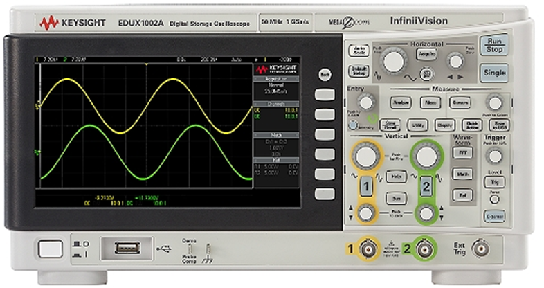
Digital Oscilloscope
Identify your workstation oscilloscope which will be used to display time-varying signals.
The input waveforms to the digital oscilloscope, sampled at 2 Giga Samples/s, are able to be stored in memory as digital words.
Advantages arise from this:
- waveforms can be stored in memory,
- more waveform measurements can be made,
- can provide screen-shot files for reports,
- can capture transient or infrequent wave-forms.
Locate the power switch (white key, bottom left) and turn the oscilloscope on.
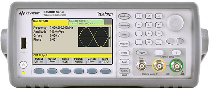
Waveform generator
Identify the waveform generator, which will be used to generate waveforms. - (Agilent 33220A still in use for some) The frequency, amplitude, offset voltage etc. may be set or varied using the front panel keys. Turn on the instrument
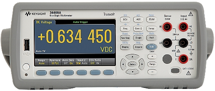
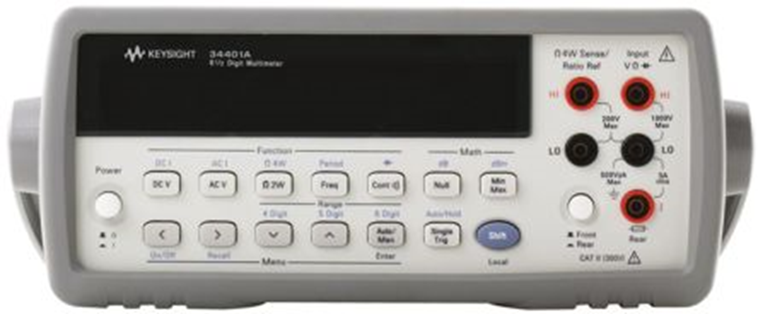
Digital Multimeter
Identify the DMM or digital multi-meter which will be used to measure voltage, current, resistance and frequency. Note that DMM input resistance is about $10 M \Omega $ when used as a voltmeter. It therefore draws minimal current when connected and has minimal effect on the active electronic or electrical circuits being measured. The signal inputs to an oscilloscope also have a very high resistance for the same reason.
Do not turn on yet.
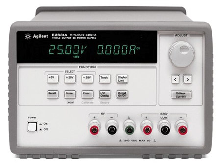
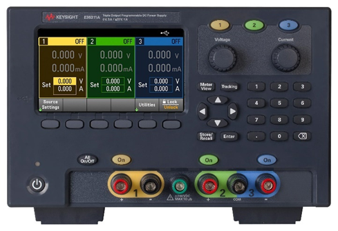
DC Power Supply
Identify the laboratory power supply that you have. Do not turn on yet. They have three variable outputs:
- +6V output, adjustable between 0V and 6V; output current up to 5A;
- +25V and –25V outputs, adjustable between 0V and 25V, output up to 1A.
Exercise 1(a)
Often the input resistance/capacitance of an instrument is recorded near the front input connections. Find these for input connections 1 and 2 of the oscilloscope. Write the answers using letters to show the power of ten multiplier and then again using scientific notation.
$R_{IN} = \qquad \qquad = \qquad \qquad \Omega$
$C_{IN} = \qquad \qquad = \qquad \qquad F$
Using the waveform generator
Power up and connection
Connect the OUTPUT of the generator to the Ch1 (channel 1) input of the oscilloscope, shown by a big 1, using a coaxial cable terminated at both end with single metal-collar BNC connectors.
To choose a waveform
When first turned on the waveform generator is set up to generate a 100mV sine-wave, but the output is not turned on. Press the Channel key above the generator Output terminal and set the Output option to on (For Agilent 33220A press Output key to turn on the o/p).
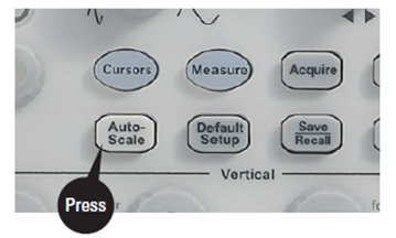
Press the white Auto-Scale key on the oscilloscope to set the oscilloscope Vertical scale [also termed gain or sensitivity (V/div)] and Horizontal [time-base ($\mu$ s/div)] scale appropriately to display the waveform
Exercise 1(b)
Use the Waveforms key and learn how to select other waveforms, from sinewave to arb and check that the correct waveform shapes being displayed on the oscilloscope for each setting?
Exercise 1(c)
What does the offset setting change with the sine-wave? What does the symmetry setting change with the ramp waveform? Select and change these settings to find out.
Setting waveform frequency
Select the sine-wave output. Press the Parameters key and select the Frequency menu soft key on bottom left.
Identify your waveform generator type and use one of the following guide boxes to adjust frequency.
The frequency value may be changed by using the upper right rotary knob and unlabelled cursor keys below the knob to change the significant digit.
Change the frequency to 1.248 kHz to practice using these keys.
It is quicker and easier to enter the frequency numerically by inputting the numbers and then selecting from the power-of-ten multipliers soft-keys.
For example, enter 12.4895 kHz using the numeric keypad buttons. First enter the digits, and then select from Hz, kHz, MHz, etc on the soft-keys.
Use the same method to change the frequency to 2.496 MHz.
Change the frequency back to 1 kHz using numerical value entry. Press AutoScale to display 2 periods.
Rotate the oscilloscope horizontal position knob, labelled ⬌ to move the waveform left or right.
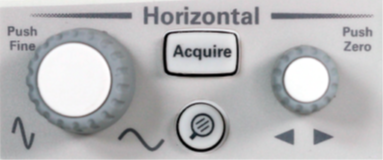
Move the waveform off-centre by several divisions (shown by the orange triangle symbol at screen top). Push in the horizontal position knob to return to zero. Rotate the yellow, channel-1 vertical position knob, labelled ⬍ ,to move the waveform up and down. Note the ground indicator ⏚ on the left also moves up and down and shows where 0 V (ground level) is located on this waveform.
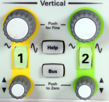
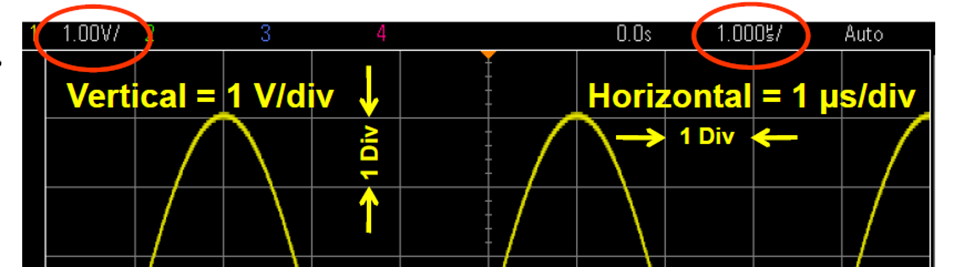
Press in the channel-1 vertical position knob to set ground (0 V) level back to the centre of the screen. Use the vertical and horizontal scales given in the Status Bar circled below to quickly measure the period, T, frequency, f, and peak-to-peak amplitude, $V_{PK-PK}$, of the sinewave and record below under Ex 2a. The horizontal and vertical position knobs may be used to better align the waveform against the centre grid lines.
Use the vertical and horizontal scales given in the Status Bar circled below to quickly measure the period, T, frequency, f, and peak-to-peak amplitude, $V_{PK-PK}$, of the sinewave and record below under Ex 2a. The horizontal and vertical position knobs may be used to better align the waveform against the centre grid lines.
Exercise 2(a)
Record the value of the waveform period and use $f=\frac{1}{T}$ to determine the corresponding frequency and then record the peak to peak amplitude.
$ T = [ \text{X-axis width of one period in div}] \times [ \text{time-base scale in $\mu$s/div} ] = \qquad = \qquad ms$
Therefore $ f = \qquad = \qquad KHz$
\(\begin{align*} V_{PK-PK} &= [\text{Y-axis peak-to-peak height of waveform in div}] \times [ \text{vertical scale in V/div} ] \\ &= \qquad = \qquad V \end{align*}\)
Exercise 2(b)
Do the measured values agree closely with the waveform generator frequency and amplitude settings?
Frequency agreement
Amplitude agreement
Setting waveform amplitude
Press the grey waveform generator Parameters key and select Amplitude on the waveform generator front panel.
The amplitude value is changed by using the rotary knob, and the horizontal arrows or by using direct numerical entry, as previously described for the frequency.
Set the amplitude to 1V PP (i.e., peak-to-peak) using numerical value entry. First enter the digits and then select the power–of-ten multiplier and signal property, i.e., peak-to-peak (PP) or root mean square (RMS). Practise amplitude entry until it’s clear. Set the peak-to-peak amplitude to 348 mV and then back to 100 mV.
Correcting the amplitude display
The waveform generator is initially set up assuming that a $50 \Omega$ load will be connected to its output, in accordance with RF (radio frequency) engineering practice of matching the waveform-generator internal $50 \Omega$ source and load internal resistance values, to maximise output signal power. Under these conditions, the waveform generator and oscilloscope give the same output voltage value. However, with a high-resistance load, such as the $1M\Omega$, oscilloscope input-channel, the values do not agree. There is an error between the displayed waveform generator voltage and the measured value on the scope.
It is necessary to change the start-up waveform-generator settings to correct this, so that the numerical display of amplitude is correctly given with a high resistance load.
Make the required correction using the following sequence of keys every time you use the waveform generator
Press the illuminated Channel key, and the following soft-key sequence:
- Output Load
- Set To High Z
- Done
Select Utility key, and the following soft-key sequence:
- Output setup
- High Z
- Done
Check that the value of peak-to-peak voltage set on the waveform-generator numerical display now agrees with that measured on the oscilloscope. If there is still an error between the peak-to-peak amplitude set by the waveform generator and your measurement, press the illuminated channel 1 key on the oscilloscope. Select Probe soft-key and change the ratio to Probe 1.00:1.
The original factory-set settings are restored when the waveform generator is switched off and next powered on. It will therefore be necessary to repeat the above key sequence each time the waveform generator is turned on unless some action is taken.
Restoring factory settings
The instrument can be put into a Store State mode, where the state of all settings previous to power-down is remembered and restored at the next power-on. This can be a nuisance when a previous user saves a series of operating settings, which you would probably not want when you come to use the instrument and turn it on. The solution is to restore the instrument to its Default Settings, i.e., restore it to a known operating status. Now that you have changed the amplitude scaling for a High Z load connection, restore the instrument amplitude scaling for $50 \Omega$ load connection by choosing Factory Settings by selecting the following key sequence:
- Press bottom, grey System key
- Select Set to Defaults
- Select Yes
- Press Store/Recall key
- Select Set to Defaults
- Select Yes
Once again set the waveform generator output to On, put the waveform generator in HIGH Z mode, set output to 100mV PP and check that the displayed amplitude approximates to the amplitude measured by the oscilloscope.
Making measurements using cursors
The oscilloscope’s cursor function will now be used to make the same voltage and time period measurements.

Press the Cursors key and experiment by pushing and rotating the adjacent knob to select and move between the two cursors sets, and to move the cursor positions.
Try to clearly understand how the cursors may be used to measure amplitude and time difference and to understand the meaning of the voltages and times listed at the bottom of the display. Discuss this with your lab partner. To aid measurement, press the Acquire key under Horizontal and select Averaging and # Avgs 8 options.
The oscilloscope computes the average of 8 screen waveforms before displaying, and so removes random noise and gives a thinner less fuzzy trace, thus allowing more precise measurement
Rotate the channel-1 (V/div) Gain knob above the illuminated 1 to increase the height of the sinewave and better fill the dis-play. Note that selection is possible between course or fine Gain (or vertical scaling) adjustment by a push-in of the Gain knob before rotating. A second push-in will return the knob to coarse adjustment. Maximise the waveform within the display area since this will allow more accurate measurement, e.g., within a $\frac{1}{4}$ or $\frac{1}{4}$ division from the top and the bottom of the display.
Exercise 3a
Using the oscilloscope cursors, measure and record the values of waveform period and peak-to-peak amplitude and use $f=\frac{1}{T}$ to determine the corresponding frequency. A div = scope grid divisions; the display has 10 horizontal & 8 vertical divisions
- $ T = \qquad ms$
- $f = \qquad KHz$
- $V_{PK-PK} = \qquad V$
Exercise 3b
To make an accurate sinewave period measurement, is it better to measure between two similar zero-crossings of the sinewave which more sharply intersect a vertical cursor line.
Exercise 3c
How might the accuracy of the sinewave period and frequency measurement be improved further?
Exercise 3d
Repeat the period and frequency measurement after making the changes previously suggested.
- $ T = \qquad ms$
- $f = \qquad KHz$
Is the result more accurate? How might the accuracy be improved even further?
Using the digital oscilloscope
Adjusting the vertical scale
Set the waveform generator to deliver a 10 kHz, 100mV pp sinewave (pp = peak-to-peak) using number entry. Press AutoScale to clearly display the waveform.
Exercise 4a
Rotate the channel-1 V/div (gain) knob fully one way and then fully the other way. Make sure you have selected coarse adjustment by pressing the Gain knob in once or twice. Record the maximum and minimum vertical scaling factors that are displayed in the top channel-status bar?
maximum $\qquad$ V/div $\qquad$ minimum $\qquad$ $\mu$V/div or mV/div
Exercise 4(b)
Using these figures, record the maximum sine-wave amplitude that can be displayed within the 8-div-high screen.
$V_{\text{max}} = \qquad V_{PK-PK}$
Exercise 4(c)
Try and set up the waveform generator to produce this large signal amplitude using number entry and describe what happens.
Adjusting the time-base and horizontal scale
Notice how, with the time-base control, you can expand or compress the time period represented by the full width of the screen, and therefore adjust the number of cycles seen on the screen. The time-base setting is shown in the status line at the top of the screen. Use this to set the time-base to 2 ms/div.
Exercise 5(a)
Given that the Ch1 waveform is a 10 kHz sine wave, calculate how many cycles of the waveform are displayed over the full width of the screen. Record your answer.
Number of cycles =
Exercise 5(b)
Calculate the time-base required to show 2 periods of the CH1 waveform within the display. Remember, $1ms = 10^{-3}s, 1 \mu s = 10^{-6}s$, therefore $1000 \mu s = 1ms$ and $1000 ms = 1s$.
Time-base = $\qquad s/\text{div}$
Set the time-base to your value and check your answer. Correct the calculation if you got the answer wrong.
The time-zero reference point of the displayed waveform, termed the trigger point, is considered to lie below the solid orange down-pointing arrow at the top centre of the screen, as indicated above.
Move the position of trigger point using the ⬌ knob at the right side of the Horizontal section.
Notice that a time is given in a pop-up display as you move the trigger point right or left.
The displayed time is the time between the new trigger point shown by the hollow orange arrow and the solid arrow at the top of the screen.
For example, with the time-base set at 20 ms/div, move the trigger point one division to the right. The actual waveform trigger point is now delayed by 20 $\mu$ s behind the screen centre; hence –20 $\mu$ s is displayed. Move the trigger point one division to the left of the centre of the screen to get a +ve or advanced 20 $\mu$ s trigger point. You can either think of the rotary knob at the right of the Horizontal section as simply a horizontal position control, or a trigger-point delay control.
You can either think of the rotary knob at the right of the Horizontal section as simply a horizontal position control, or a trigger-point delay control.
Run Controls
Reset the waveform generator frequency to 1 KHz.
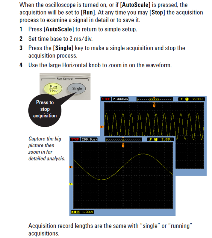
Press AutoScale to return to a simple set-up.
Oscilloscope trigger controls
You can think of oscilloscope “triggering” as “synchronized picture taking”. When an oscilloscope is capturing and displaying a repetitive input signal, it may be taking tens of thousands of pictures per second of the input signal. In order to view these waveforms (or pictures), the picture-taking must be synchronized to “something”. That “something” is a unique point in time on the input signal.
An analogous situation to oscilloscope triggering is that of a photo finish of a horse race. Although not a repetitive event, the camera’s shutter must be synchronized to the first horse’s nose at the instant in time that it crosses the finish line. Randomly taking photos of the horse race sometime between the start and end of the race would be analogous to viewing un-triggered waveforms on a scope.
To understand oscilloscope triggering, set the waveform generator to High Z mode and set the output to $2V_{PK-PK}$, 1kHz sinewave.
- Press Default Setup on the scope’s front panel and select Factory Default/OK.
- Press channel 1 key in yellow area and change the probe scaling from 10:1 to 1:1.
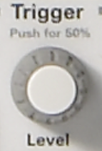
- Press the Trigger front panel key below the trigger level knob.
- Press the Trigger Type softkey. Your scope display should now look similar but not exactly the same as .
Using the scope’s default trigger conditions, the oscilloscope should be triggering on a rising slope as the signal crosses the 0.0 V trigger level in the centre of the screen as below.
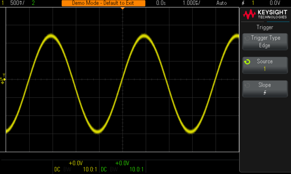
Use the trigger menu Slope soft-key to change to the Falling slope and note the falling slope of the sinewave is now synchronised to the centre of the screen.
The point in time shown at the screen centre (both horizontally and vertically) constitutes the trigger reference point, i.e., zero-time reference 0.0 seconds, and the trigger level 0.0.
The solid orange triangle trigger-point is the point about which the waveform will expand or contract when the scope time base is changed.
Rotate the time base knob to observe how the waveform expands or contracts about this fixed point, which means a wave-form’s reference position does not have to be constantly adjusted after a change in time base.
It is also possible to trigger the scope on a feature of a waveform, e.g., a glitch, so that the region of a waveform may be expanded while remaining fixed centre screen for more detailed investigation.
Rotate the trigger level knob clockwise to increase the trigger level voltage.
Rotate the trigger level counterclockwise to decrease the trigger level voltage setting.
As you increase the trigger level voltage setting, you should observe the sinewave shifting in time to the left.
If you decrease the trigger level voltage setting, the sinewave will shift to the right.
Adjust the trigger level knob and note a horizontal line shows where the trigger level cuts the waveform.
Note the exact trigger voltage setting is always displayed in the upper right-hand corner of the display.
If you stop rotating the trigger level knob, the orange trigger level line will time-out and disappear after a few seconds, but there is still a yellow trigger level triangle and T shown on the left, outside the waveform graticule area, to indicate where the trigger level is set relative to the waveform. It may be shown on top of the waveform 0V position symbol if the trigger level is also 0V.
Increase the trigger level voltage setting until the orange level indicator is above the peaks of the sine wave.
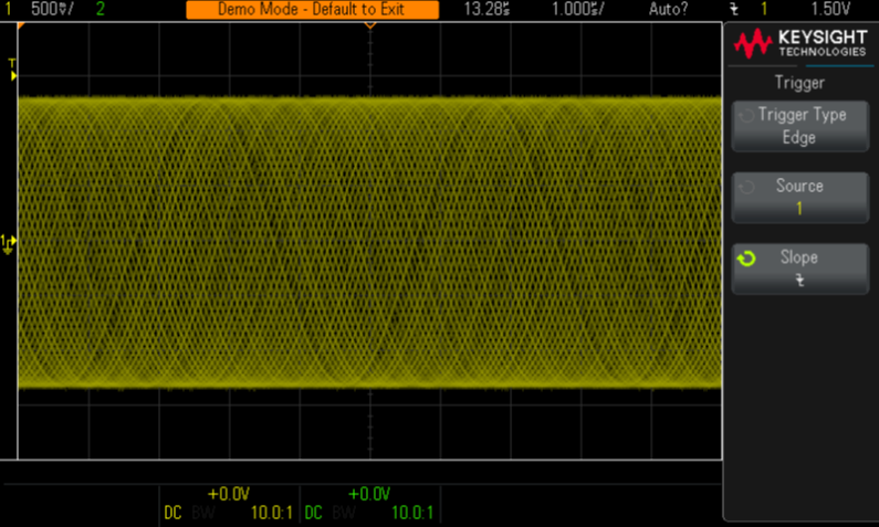
With the trigger level set above the sine wave, the scope’s waveform display is no longer synchronized to the input signal, since at this particular trigger level setting the trigger level no longer intersects the wave-form. Your scope’s display should now look similar to . The scope is now “auto triggering”.
Auto Trigger is the scope’s default trigger mode. In Auto Trigger mode, if an input signal does not intersect the trigger level, then the scope will generate its own asynchronous trigger and begin displaying pictures (acquisitions) of the input signal at times set by an internal timer. Since the “picture taking” is then no longer synchronised with the waveform, a set of waveforms is captured and over-layed at different positions in the display. This blurring is a clue that scope acquisition is not triggering on the input signal, or synchronised to it, and the trigger level or trigger settings need to be adjusted.
Push the Trigger Level knob once to reset the trigger level to 0.0 V and properly trigger waveform capture.
Trigger edge
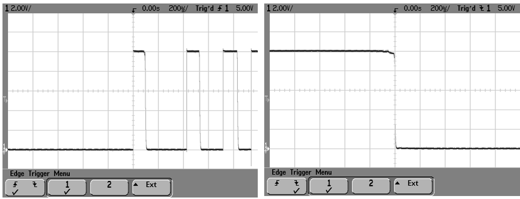
Exercise 6(a)
Sketch waveforms to show how the square-wave and saw-tooth/triangular waveforms will be aligned with the centre of the screen for both rising and falling trigger edge settings.
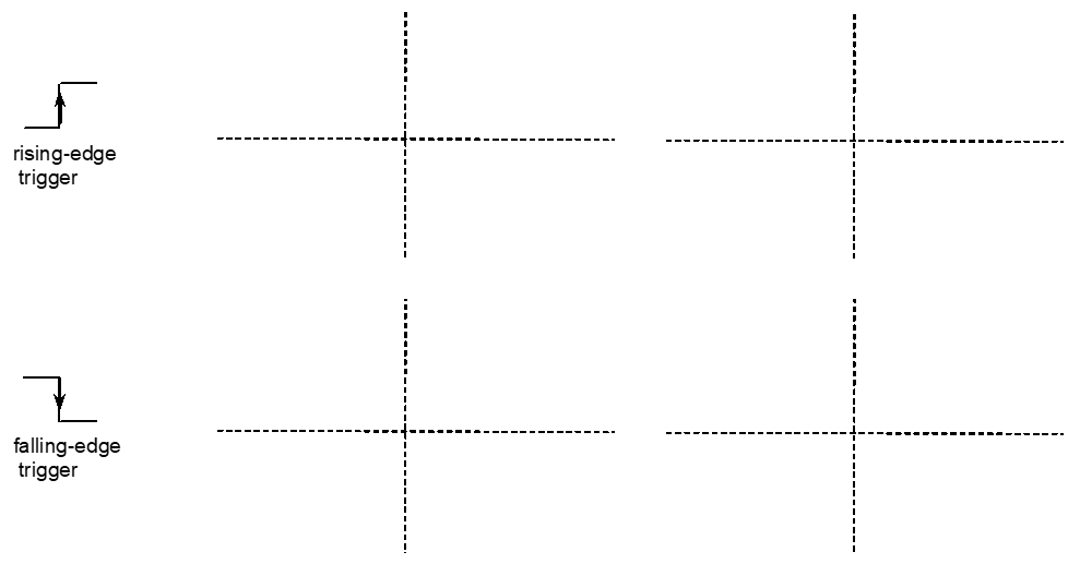
Set the waveform generator to output each of the waveforms on the waveform generator and use Auto Scale and different Trigger / Trigger Type / Edge settings within the Trigger menu to check your predictions.
The Normal trigger mode is used when a trigger event occurs very infrequently (including transient or single-shot events). For example, to display a very narrow infrequent 1Hz or once per second pulse. If the scope’s trigger mode was set to the Auto trigger mode, the scope would generate lots of asynchronously generated automatic triggers and would not be able to show the infrequent narrow pulse. Therefore, the Normal trigger mode would be selected so that the scope would wait until obtaining a valid trigger event before displaying waveforms.
Set the waveform generator to produce a 1 Hz, 200 mV, 100 $\mu$ s pulse.
Adjust the oscilloscope’s channel 1 time-base and gain settings to 100 $\mu$ s/div and 50mV/div, respectively, and set the trigger level to 0 V. Press the Trigger key and check the Mode is set to Auto.
Exercise 6(b)
Is the $100 \mu s$ pulse visible on the oscilloscope’s display? Describe what you see.
Exercise 6(c)
Explain how the infrequent pulse waveform may be clearly displayed on the oscilloscope.
Exercise 6(d)
Press the Trigger key and make an appropriate change to the settings so that a steady pulse waveform is displayed. Expand the pulse and measure the approximate pulse rise time.
Exercise 6(e)
Make an appropriate change to the Trigger settings so that you can also measure the and fall time
- $T_{RISE} = \qquad ns$
- $T_{FALL} = \qquad ns$
Automatic voltage and time measurements
Set the waveform generator to give a 10kHz, 4V peak-to-peak sinewave output.
Press Default Setup on the scope’s front panel and select Factory Default/OK to reset the scope to a known state. Set channel 1 Probe scaling from 10:1 to 1:1 and then press Auto Scale.
Press Measure and note that the frequency and peak-to-peak magnitude of the channel1 signal are displayed at the bottom of the screen.
Multi-meters that electricians use to measure the 50HZ AC mains supply voltages, measure the root mean square value of a sinewave, since it is easier to measure than the peak sinewave voltage and the square is directly proportional to power as in $P=\frac{V^2}{R}$.
To measure RMS voltage, press Measure and set Type to DC RMS-Full Screen. The DC RMS-FS(1) value for a 4V peak-to-peak sinewave should correspond close to $V_{RMS}= V_{PK-PK} (2/ \sqrt{2}) = 4/(2 \sqrt{2}) = 1.41V$ and should be shown at the bottom right of the screen.
Exercise 7(a)
When making measurements on waveforms or doing a screen dump to a USB flash memory drive to include a waveform copy in a report, what is the best way to show the waveform in the display?
Choose one of the following:
- one clear cycle
- several clear, contrastable cycles
- an impressive blur of tens perhaps even hundreds of cycles.
Choose one of the following:
- a narrow strip of vertically compressed space-saving waveform
- a big, unmissable display of clipped waveforms
- a modest number of waveforms that fit comfortably with-in the oscilloscope display frame.
Exercise 7(b)
Change the oscilloscope gain and time base to comply with your above decisions. Record the pk-to-pk and RMS values.
- $V_{PK-PK} = \qquad V$
- $V_{RMS} = \qquad V$
Turn off and disconnect the waveform generator which will not be used in the next section.
Using the digital multimeter (DMM) and power supply
Connecting and setting up the power supply
Collect a 47 $\Omega$, 25W power resistor mounted on an aluminium heat sink, which is connected in series with a switch. Connect it directly into the +25V +VE and Com terminals of the Agilent E3631A power supply so it hangs down.
Connect the black and red gripper leads directly across the resistor, using the wire loops connected to the resistor terminals, and connect the 4mm plugs at the other end of the leads to the red V$\Omega$ and black to LO on the right side of the DMM front panel. The DMM will now be used to measure resistor voltage.
Turn on the power supply and DMM by pressing the Power keys.
Press the DC V key of the DMM to measure DC voltage.
Turn on the power supply outputs by pressing the Output On/Off key
Press the **+25V key and increase the voltage using the rotary knob to 10V.
Notice that the power-supply display shows the voltage and current delivered by the selected outputs. If the current is zero you may have to change the position of the switch in series with the resistor to close the circuit.
Exercise 8(a)
Record the values of the current (I) and the voltage (V) now delivered to the resistor (i.e. the values shown on the power supply display).
- $V_R = \qquad V$
- $I_R = \qquad A$
Exercise 8(b)
Given Ohm’s Law, i.e. $R = \frac{V}{I}$, use the V and I values to calculate the value of resistance.
$R_{\text{Measured}} = \qquad \Omega$
Exercise 8(c)
Is this the value that you expected given the component details on the body of the resistor, i.e., $R_{\text{Nominal}}$? Read all the details on the resistor and try to explain the value obtained.
Exercise 8(d)
Calculate the percentage error in the resistance. The % error is given by the following equation.
\(\frac{R_{\text{Measured}} - R_{\text{Nominal}}}{R_{\text{Nominal}}} \times 100 \text{ or with a change } \frac{R_{\text{New}} - R_{\text{Old}}}{R_{\text{Old}}} \times 100 = \qquad \%\)
Exercise 8(e)
State the advantage of calculating error (or change) as above and including a sign as well as a % difference. Is your resistor within the specified manufacturing tolerance of $\pm 5 \%$.
To measure resistance using the DMM
Press the power supply Output On/Off key to turn the outputs off.
Disconnect the resistor from the power supply: you should never try and measure resistance in a live circuit.
Connect the resistor with the switch in the closed position between the $V \Omega$ and LO inputs of the DMM and select $ \Omega 2 W$ to measure resistance directly.
Exercise 9(a)
Record the resistance given. The value should be in good agreement with the value determined early from V and I measurement. Check that this is the case.
$R_{\text{Ohmmeter}} = \qquad \Omega$
% Difference from value by V-I measurement =
Exercise 10(a)
Use the DMM configured as an Ohmmeter to measure the resistance values of the two low-power resistors provided.
- $R_1 = \qquad \Omega$
- $R_2 = \qquad \Omega$
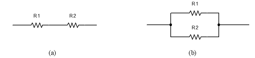
Exercise 10(b)
Connect the two resistors in series as shown in by twisting two of the resistor leads together and measure and record the total resistance between the outside leads. Record the value as $R_s$.
$ R_s = \qquad \Omega$
Exercise 10(c)
Connect the two resistors in parallel as shown in by twisting adjacent pairs of the resistor leads together and measure and record the total resistance between the leads. Record the value as $R_p$.
$R_p = \qquad \Omega$
Exercise 10(d)
Check, by submitting $R_1$ and $R_2$ into the following equations, which give the total resistance for the series and parallel connections, that the values of $R_s$ and $R_p$ are in good agreement with those just measured.
- $R_s = R_1 + R_2 = \qquad \Omega$
- $R_p = \frac{R_1 R_2}{R_1 + R_2} = \qquad \Omega$
To measure AC voltage using the DMM
The DC power supply is not used and should remain off. Press the AC V key on the DMM to measure AC voltage.
Connect the DMM ($V \Omega$ and LO terminals) and oscilloscope across the output of the Waveform Generator using the coaxial T-piece connector and the coaxial lead with BNC and 4mm connectors.
Set the waveform generator to give a 1kHz.
Press the Waveform Generator Ampl key and enter 1 V RMS (not 1V pk-pk this time) by pressing Enter Number, 1, and finally the down arrow with VRMS beside it.
The DMM displays the root-mean-square, RMS, value of an AC waveform since the power delivered by an AC waveform is given by the RMS value as with a constant DC voltage, using $P = \frac{V_{RMS}^2}{R} $.
For sinewaves, the RMS value is obtained from the peak value by dividing by root 2 (note peak-to-peak values must first be divided by 2 to get the peak value). $ V_{RMS} = \frac{V_{PK}}{\sqrt{2}} = \frac{V_{PK-PK}}{2} \times \frac{1}{\sqrt{2}}$
If you have succeeded, the waveform generator will display 1.000 VRMS, and the value displayed on the waveform generator and DMM should be in good agreement.
Observe the waveform on the oscilloscope with a vertical and scale of 500 mV/div. Make sure the channel 1 probe scaling ratio is set to 1:1 and not 10:1 from X10 to X1, so that the full waveform can be seen.
Exercise 11(a)
By using the scope Measure facility on the oscilloscope, selecting the RMS option rather than peak-to-peak measurement option, and changing the time-base for each setting to display several cycles, quickly complete the table below.
| Frequency (MHz) | Waveform Generator AMPL (V RMS) | DMM AC V (V RMS) | Scope Quick Measure RMS MEASURE (V RMS) |
|---|---|---|---|
| 0.1 | 1 | ||
| 0.3 | 1 | ||
| 0.5 | 1 | ||
| 1 | 1 | ||
| 2 | 1 | ||
| 5 | 1 | ||
| 10 | 1 | ||
| 15 | 1 |
Exercise 12(a)
Comment on which instrument you believe makes the most accurate AC voltage measurement (i) below 1 MHz (ii) above 1MHz? Note that the actual signal generator waveform is modified by the coaxial cable impedance (largely capacitance) and hence there is actually some signal attenuation between the source circuit and measurement points.
-
Below 1 MHz
-
Above 1 MHz
Advanced exercises for later or if you finish previous work early
Display of single shot waveforms
Connect the $47 \Omega$ resistor and switch assembly across the +25V output of the power supply.
Select the +25V output and switch it on using the Output On/Off key. Adjust the voltage to 10V. Connect the oscilloscope probe BNC connector to Ch1, and the probe tip and crocodile clip directly across the power resistor using the wire loops near the resistor terminals. Make sure the probe crocodile clip is connected to the power-supply COM side.
Press Default Setup on the scope’s front panel and select Factory Default/OK to reset the scope to a known state. Leave channel 1 Probe scaling at 10:1 and set the scope probe slider switch to 10:1 signal scaling.
Position the Ch 1 zero-level symbol to 1 div from the base of the screen using the Ch 1 position knob, and set the vertical scale to 2 V/div and the time base to 200 $\mu$s/div.
Turn on and off the switch connected to the resistor to identify which position is on and which is off. In the on position, the scope trace should jump up 5 divisions to indicate that the probe is measuring a DC level of 10V.
Set the trigger level to 5V within the Waveform section. Make sure that the trigger Mode/Coupling key is set to Normal within the trigger Mode menu.
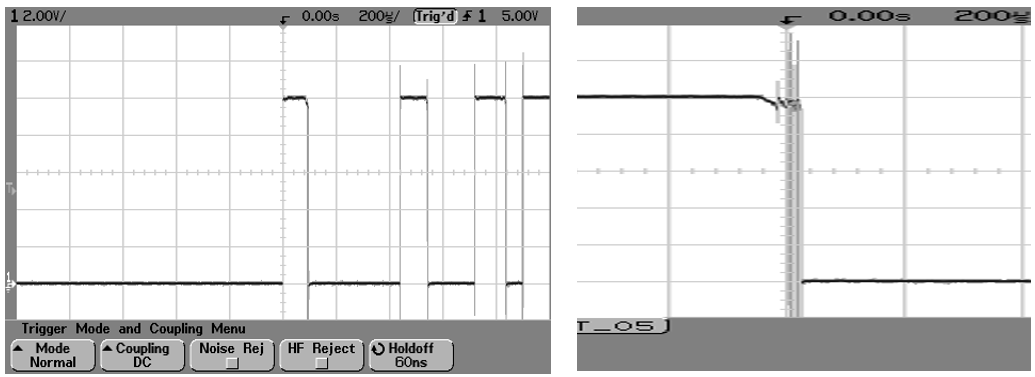
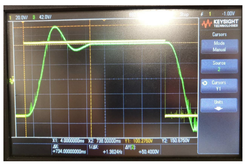
Turn the resistor switch on and off and you should capture a switching transient each time the switch is toggled which is something like one of the waveforms shown in .
If you have difficulty obtaining traces like those shown in , you may have to press the Single key in the Run Control section prior to each change in switch state.
The switch contacts bounce several times before finally staying in either an open or closed state after switching. This contact bounce is most evident in the turn-on switching transition in . The pattern of pulses tends to vary each time the switch is thrown.
Change the time base setting to 100 ns/div and change the trigger edge to falling in the Edge menu.
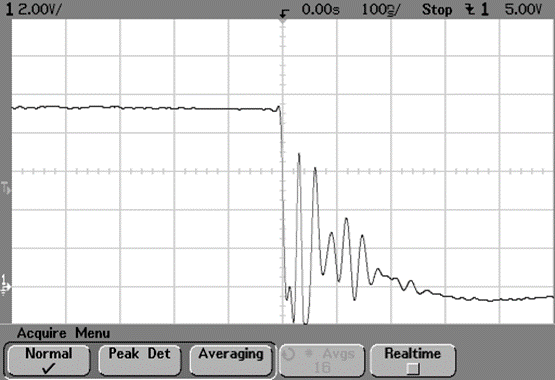
Exercise 14(a)
Use the oscilloscope cursors to measure the frequency of the damped ringing captured during switch turn off. Record the value obtained.
Switch off the output of the power supply using the Output On/Off key and connect a 0.1 $\mu$F capacitor directly across the switch contacts by inserting it into the grey terminal block.
Turn the power supply output back on, operate the switch and capture the new switching transient as you increase the time base from 5 $\mu$s/div to 200 $\mu$s/div.
Amplitude modulated signal
Set the waveform generator to output an amplitude-modulated 500KHz, 2V signal.
Exercise 16(a)
Set up the oscilloscope to display several modulating signal periods of the waveform. The modulating signal cycles should be rock steady in the display.
Key settings used:
Saving the oscilloscope display for reports
The oscilloscope had a USB type A port which may be used to create screen-shot image files to include in reports.
Exercise 17(a)
Investigate saving the display file to your flash memory drive and then inserting the image file into a Word document. Press scope top right Run/Stop key to freeze a waveform in the display. Insert your USB memory stick. Press the oscilloscope Save/Recall key and choose Save on the left black screen.
- Press the Format Setup softkey and set as PNG.
- Press the Save To softkey to select a USB directory if different from the root directory.
- Use Press to Save softkey to save the waveform.
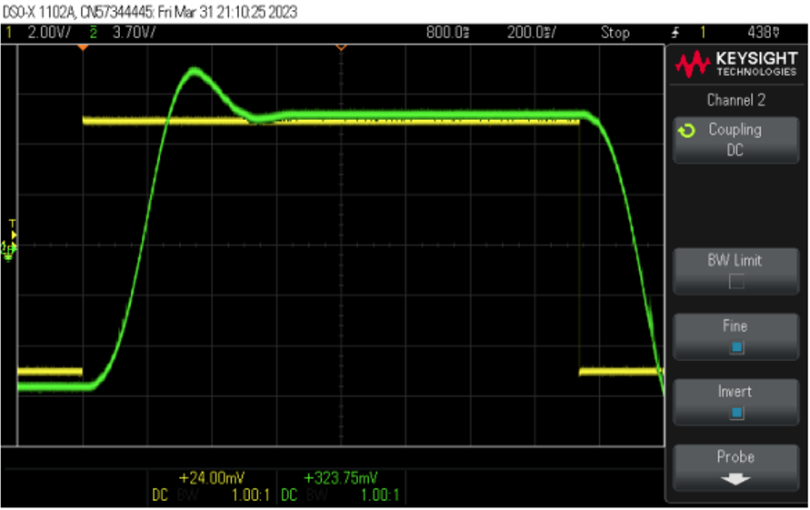
Note the scope traces may be set to be black on a white background using the Settings softkey options. Check the display files by inspecting on a desktop PC or by inserting into a Word document
When capturing scope screen copies for reports, it is generally better to insert a downloaded scope png file in a report (first image below). The alternative of using or a phone-camera-shot (second image below) often results in poor clarity of some of the essential scope set-up data. What is required to download scope images?
References used in preparing these lab notes.
- Keysight Technologies, Resource Center Document Library, Retrieved July 14. 2018 from: https://www.keysight.com/en/pdx-2766199-pn-DSOX1102A/oscilloscope-70-100-mhz-2-analog-channels?cc=US&lc=eng
- Keysight InfiniiVision 1000 X-series Oscilloscopes, User’s Guide, Manual Part Number 54611-97000, Keysight Technologies, Inc, Colorado Springs, CO 80907, 2nd Edition, Feb 2018.
- Educator’s Training Kit for 1000 X-series Oscilloscopes, Manual Part Number 54612-97015, Keysight Technologies, Inc, Colorado Springs, CO 80907, March 2017.