Be sure to do all exercises and run all completed code cells.
If anything goes wrong, restart the kernel (in the menubar, select Kernel\(\rightarrow\)Restart).
Statistical Data Analysis
This section is using some of the skills you’ve learned to perform data analysis, which is an important use of coding and using the Pandas data analysis library and Numpy.
Watch the two video lectures on statistics then work independently on coding up the parameters shown in the videos in the parts below.
Submit parts 1\(-\)3 in a single python script (worth 3%)
Part 1 (1%)
Read in
Files/soil_regression.xlsxTake out the
"PI (%)"column as \(x\) values and the"CBR (%)"column as \(y\) valuesCalculate the fitting parameters
a0anda1
# Part 1
# YOUR CODE HERE
Run the cell below to check your values of \(a_0\) and \(a_1\)
print(a0, a1)
Expected result:
5.304019... -0.112705...
(these will be checked by the marking script with more decimal places)
Part 2 (1%)
Write a function that returns a predicted \(y\) value based on a new \(x\) value, based on the linear model \(\widehat y = a_0 + a_1 x\)
# Part 2
# YOUR CODE HERE
Run the cell below to check your function
xnew = 30
ypred = prediction(a0, a1, xnew)
print(ypred)
Expected result:
1.922861...
(this will be checked by the marking script with extra decimal places)
Part 3 (1%)
Using the array of
PI (%)measurements as the \(x\) values, calculate an array of model \(\widehat y\) values, given by the linear model \(\widehat y = a_0 + a_1 x\)Calculate the coefficient of determination (goodness of fit) based on the equation at the end of the second statistics lecture:
# Part 3
# YOUR CODE HERE
print(r2)
Expected result:
0.457818...
(this will be checked by the marking script with extra decimal places)
Extra (for fun)
Part A
Put the (rounded) model \(\widehat y\) values back into the DataFrame
Sort the DataFrame by the
"PI (%)"column
# YOUR CODE HERE

data
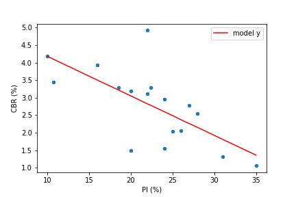
Expected format:
sample |
PI (%) |
CBR (%) |
model y |
|---|---|---|---|
\(\bf 4\) |
10.0 |
4.18 |
4.18 |
\(\bf 10\) |
10.7 |
3.45 |
4.1 |
\(\bf 11\) |
16.0 |
3.94 |
3.5 |
\(\bf 12\) |
18.5 |
3.28 |
3.22 |
\(\bf 20\) |
20.0 |
1.5 |
3.05 |
\(\bf 6\) |
20.0 |
3.2 |
3.05 |
\(\bf 15\) |
22.0 |
4.92 |
2.82 |
\(\bf 18\) |
22.0 |
3.12 |
2.82 |
\(\bf 16\) |
22.4 |
3.28 |
2.78 |
\(\bf 7\) |
24.0 |
1.56 |
2.6 |
\(\bf 13\) |
24.0 |
2.95 |
2.6 |
\(\bf 3\) |
25.0 |
2.03 |
2.49 |
\(\bf 9\) |
26.0 |
2.05 |
2.37 |
\(\bf 5\) |
27.0 |
2.79 |
2.26 |
\(\bf 8\) |
28.0 |
2.54 |
2.15 |
\(\bf 19\) |
31.0 |
1.31 |
1.81 |
\(\bf 2\) |
35.0 |
1.06 |
1.36 |
Finally
Various libraries can be used to do the tasks for you.
Fitting
import numpy as np

xvals,yvals = np.loadtxt("Files/soils.csv", delimiter=',', skiprows=1).transpose()[1:3]

degree = 1 # 1D "linear" fit
m, c = np.polyfit(xvals, yvals, degree)

print(c, m)
Compare these values with the ones you got in Part 1
Coefficient of determination
In Numpy you can use the correlation coefficient function:
corrs = np.corrcoef(xvals, yvals)

print(corrs**2)
Compare the value at index
[0,1]to your \(R^2\) calculation in Part 3
Another way is using the Scientific Python scipy library
from scipy.stats import linregress

slope, intercept, r_value, p_value, std_err = linregress(xvals, yvals)

print(r_value**2, intercept, slope)
Or even a simple function in the powerful machine learning library sklearn
from sklearn.metrics import r2_score

ypred = slope*xvals+intercept
print(r2_score(yvals, ypred))