Be sure to do all exercises and run all completed code cells.
If anything goes wrong, restart the kernel (in the menubar, select Kernel\(\rightarrow\)Restart).
2-Dimensional Arrays, Dictionaries and DataFrames
Let’s explore some useful data types and new ways of interacting with data.
Numpy N-D arrays
http://docs.scipy.org/doc/numpy/reference/arrays.ndarray.html
You have seen that numerical arrays from NumPy can be more than a one-dimensional column. There are various ways to create an array, including converting from a list, entering all the values by hand, or generating large arrays using special functions and loops. We can also change the individual values in arrays.
Study the following examples and practice changing things and looking at the outputs to understand how things work.
Converting from a list to an array
If we have all the values in a (nested) list it can be converted to a numerical array:
import numpy as np

mylist = [[1,2,3],[4,5,6],[7,8,9]]

myarray = np.array(mylist)

print(myarray)
An array has a dimension and a shape:
print(myarray.ndim)
print(myarray.shape)
This means it is a 2 dimensional array, with 3 rows and 3 columns.
Accessing array values by index
We can also access the elements of square arrays using indexing: arrayname[row,col], where the variables row and col are replaced by the values of the row and column number we want to access.
print(myarray[0, 2])
Print the middle number in the block (5).
# myarray[?, ?]
# YOUR CODE HERE
Print the last number in the block (9)
# YOUR CODE HERE
To change a value
myarray[1, 1] = 111

print(myarray)
Manipulating numerical arrays
http://docs.scipy.org/doc/numpy/reference/routines.array-manipulation.html
Generating Arrays using Special Functions
nrows = 5
ncols = 7
dimensions = (nrows, ncols)
myzeros = np.zeros(dimensions)
print(myzeros)
Try using different numbers for the parameters in these functions to see what happens.
from numpy.random import random
dims = (5, 2)
rands = random(dims)
randr = rands.round(2)
print(randr)
Shorthand notation can also be used:
myzeros = np.zeros((nrows,ncols))
We can take slices of an array using the notation arrayname[ROWSLICE, COLSLICE], where ROWSLICE and COLSLICE use the same slicing rules STARTAT:ENDBEFORE as seen in previous sections.
For example we can slice off a single row or column:
The code below does the following:
Create an array of ones using the
numpy.onesfunction with one column and five rows.Change the middle value to 5.
slice the column into the middle column of an array of \(5\times7\) zeros.
myones = np.ones((5,1))
print(myones)
myones[2] = 5
print(myones)
newarray = np.zeros((5, 7))

newarray[:, 3] = myones[:, 0]
print(newarray)
Note that
myonesis a 2D array so we have to slice all values:in column0using[:, 0]
Further reading can be found here.
Import an Export of N-D data using NumPy
Load a column of text from the file "temps.txt" into an array using the ARRAY=np.loadtxt(FILENAME) method.
Python Dictionaries
A dictionary of keys or dict is a data type with pairs of KEY:value entries. They are defined in curly brackets and the values can be different types. For example:
fruit={"apple":"A red fruit.", "banana":"A yellow fruit.", "tomato":"A red fruit."}
You can then look up (or change) an item’s value in the dictionary using its key:
fruit["banana"]
fruit["apple"] = "A red or green fruit."

fruit["apple"]
New entries can also be added:
fruit["aubergine"] = "A purple fruit"

fruit
The values can also be numerical, allowing us to count things:
eggs={} #we can start with an empty dict
eggs["hen"]=1 #if the key does not exist it is added to the dictionary
eggs["duck"]=5
print(eggs)
eggs["hen"]+=1 # += is a shorthand for "add one to the value"

print(eggs)
Entries can also be lists or arrays (or any other object)
thedata = dict() #another way of making an empty dictionary

thedata["Days"] = list(range(1,8))
thedata["Temperatures"] = np.array([23.3, 16.9, 21.8, 26.9, 23.5, 21.7, 19.8])

thedata
Which can also be manipulated:
thedata["Temperatures"] = thedata["Temperatures"]-10

thedata["Temperatures"]
Data Frames and Pandas
Pandas is a very powerful data analysis library that extends on the functionality of numpy and matplotlib.
It can be used to load, analyse plot and save data.
See the comprehensive cheatsheet on moodle for full information about Pandas
The basic data types used by pandas are the dataframe and the series. Here we’ll look at dataframes, which are 2D arrays with labels and related to a spreadsheet.
import pandas as pd

# make a dataframe called df out of our previous dictionary:
df = pd.DataFrame(thedata)
print(df)
In Jupyter-Notebooks dataframes will display with nice formatting by putting just their name at the end of a code cell:
df
Columns can be accessed in the same way as dictionaries:
df["Temperatures"]
And they can be manipulated like Numpy arrays:
average = df["Temperatures"].mean()
print(average)

deviation = df["Temperatures"]-average
print(deviation)
As well as writing new columns:
df["Deviations"] = deviation

df
This can then be saved as a CSV using df.to_csv("<FILENAME>.csv") or even an Excel spreadsheet:
Note: the
index=Falseargument makes sure the left-hand index column ([0,1,2,3,4,5,6]) does not get written to the spreadsheet.The
sheet_nameargument allows you to name the sheet tab in Excel.
df.to_excel("devdata.xlsx", index=False, sheet_name="Temperature Deviations")
Now download and open the
devdata.xlsxfile that was just created!
Lists and arrays can also be used to make Data-Frames:
import numpy as np
import pandas as pd

temps = np.array([23.3, 16.9, 21.8, 26.9, 23.5, 21.7, 19.8])
average = temps.mean()
devs = temps-average # deviation of each point from the mean
stdev = temps.std() # standard deviation of the dataset
zscore = devs/stdev # Z-score is the number of standard deviations each reading is from the mean
data = [temps, devs, zscore]

mynewdataframe = pd.DataFrame(data)
mynewdataframe
# rotate the dataframe:
newdata = mynewdataframe.transpose()
newdata
Data can be accessed and manipulated in similar ways to 2D arrays, but also accessed by the column name, new columns can be inserted etc.
A dataframe also has an object variable .columns inside which describes the column headings.
In the above example
newdata.columns = [0, 1, 2]by default.
Renaming the columns
newdata.columns = "Temp", "Deviation", "Z-value"

newdata
A dataframe also has a .index property naming the rows, which can be changed:
newdata.index = ["Mon", "Tue", "Wed", "Thu", "Fri", "Sat", "Sun"]

newdata
See the very comprehensive sheet on moodle (also ones such as this one) to find out more details.
Importing spreadsheet data
It is possible to import data into a data-frame from plain text files, CSV files or even excel spreadsheets.
import pandas as pd

data = pd.read_excel("Files/Case Study Data.xlsx", sheet_name="Data")

data
Individual columns can be extracted using the following syntax:
projects = data["Project"]

print(projects)
And subsets can be pulled from the data and made into their own dataframe.
selected_columns = ["Total.Area.sqm", "Cost.Million.USD"]

data2 = data[selected_columns]

data2.index = projects # from the previous cell

data2
import pandas as pd

data = pd.read_excel("Files/Case Study Data.xlsx", sheet_name="Data")

cost = data["Cost.Million.USD"]
area = data["Total.Area.sqm"]
costpermetre2 = cost/area

# create a new column
data["Cost.Per.sqm"] = costpermetre2


selected_columns = ["Project", "Total.Area.sqm", "Cost.Million.USD", "Cost.Per.sqm"]

# create a new DataFrame with the selected columns as the data and set the project name column as the index
newdata = data[selected_columns].set_index("Project")

newdata
Pandas is very good at plotting the data.
ax = newdata["Total.Area.sqm"].plot(kind="bar", figsize=(15,5)) # returns a set of figure axes
Different plot styles are available
ax1 = newdata["Total.Area.sqm"].plot.hist(edgecolor="black")
ax2 = newdata.plot.scatter(x="Total.Area.sqm", y="Cost.Million.USD")
Plots can be saved or manipulated using this method:
ax2.figure.savefig("scatterplot.png") # how to access the figure canvas and save it
And plots can appear on the same axes or in subplots.
sortdata = newdata.sort_values(by="Total.Area.sqm")

ax3 = sortdata.plot.bar(subplots=True, figsize=(15,9))
Filtering data:
Data can also be filtered in the following way:
costmilUSD = data2["Cost.Million.USD"] #select the column

condition = costmilUSD>100 #filter selected values

data3 = data2[condition]

data3
Try breaking this down and printing each line to see what’s going on in each step.
This can then be combined into a single line, which is more compact but harder to read.
data3 = data2[data2["Cost.Million.USD"]>100]
New columns can also be created by doing calculations on existing ones:
Pivoting Data
The data can also be pivoted, like in Excel:
import pandas as pd

data = [["A", "T-1", 0.1],
        ["A", "T-2", 0.2],
        ["A", "T-3", 0.3],
        ["B", "T-1", 0.4],
        ["B", "T-2", 0.5],
        ["B", "T-3", 0.6],
        ["C", "T-1", 0.7],
        ["C", "T-2", 0.8],
        ["C", "T-3", 0.9]]

df = pd.DataFrame(data)
df.columns = "Class", "Type", "Value"
df
Pivoting uses the DataFrame.pivot(index, columns, values) function method,
index : Column to use to make new frame’s index.
columns : Column to use to make new frame’s columns.
values : Column(s) to use for populating new frame’s values.
piv = df.pivot("Class", "Type", "Value")
piv
Exercises for Weekly Task (2%)
Use the above notes and cheatsheets/online help to guide you through.
There are no model answers given as this builds into the mini-coursework for this lesson.
You will need to refer to both the notes and the Pandas pdf cheat sheet(s) and online resources to do these exercises
Work through the exercises in Jupyter-notebook as you do the task step-by-step.
Once complete copy the code in the numbered blocks to a single python
.pyscript for submission.
Part 1
Read in the csv file
"energy.csv"as a dataframe nameddata.You must have the input file in the current working folder.
#Part 1
import pandas as pd

# YOUR CODE HERE
Run the next cell to check what was created:
print(data.head()) #your dataframe should look like this:
Expected Result:
   month  day  hour  elec   gas
0      1    1     1   0.0  0.746
1      1    1     2   0.0  0.672
2      1    1     3   0.0  0.075
3      1    1     4   0.0  0.141
4      1    1     5   0.0  0.078
Part 2
Make a new column called
totalthat is a sum of the “elec” + “gas” columns
# Part 2

# YOUR CODE HERE
# check result
print(data.head())
Expected Result:
   month  day  hour  elec    gas  total
0      1    1     1   0.0  0.746  0.746
1      1    1     2   0.0  0.672  0.672
2      1    1     3   0.0  0.075  0.075
3      1    1     4   0.0  0.141  0.141
4      1    1     5   0.0  0.078  0.078
Part 3:
Select only Day 21 of each month.
Make a new dataframe
selectedthat is only filtering rows ofdatawhere thecondition = (days==21)Use the notes here to help you.
# Part 3
# YOUR CODE HERE
# check the result
selected
Expected result:
     month  day  hour   elec    gas  total
480      1   21     1  4.884  0.557  5.441
481      1   21     2  0.000  0.323  0.323
482      1   21     3  0.000  0.077  0.077
483      1   21     4  0.000  0.056  0.056
484      1   21     5  0.000  0.115  0.115
       month  day  hour   elec    gas  total
8515     12   21    20  6.409  1.520  7.929
8516     12   21    21  5.494  0.763  6.257
8517     12   21    22  6.714  1.035  7.749
8518     12   21    23  5.799  0.981  6.780
8519     12   21    24  5.493  1.096  6.589
Part 4: Pivot the data into a table of totals for each hour and month
use
"hour","month","total"as the COL, ROW, DATA arguments in the.pivot()function
# Part 4

# YOUR CODE HERE
# check result

piv.head()
Expected Result:
month     1      2      3      4      5      6      7      8      9      10   ...
hour
1      5.441  4.521  0.392  0.200  0.357  0.162  0.200  0.131  0.101  0.141   ...
2      0.323  0.104  0.056  0.136  0.048  0.072  0.150  0.149  0.120  0.099   ...
3      0.077  0.050  0.093  0.128  0.115  0.136  0.122  0.107  0.120  0.091   ...
4      0.056  0.107  0.072  0.131  0.075  0.099  0.094  0.098  0.104  0.098   ...
5      0.115  0.045  0.056  0.133  0.085  0.093  0.146  0.043  0.093  0.104   ...
...
Part 5:
Change the column titles to "Jan", "Feb", "Mar", "Apr", "May", "Jun", "Jul", "Aug", "Sep", "Oct", "Nov", "Dec"
# Part 5

# YOUR CODE HERE
# check the result
print(piv.head())
        Jan    Feb    Mar    Apr    May    Jun    Jul    Aug    Sep    Oct   ...
hour                                                                         ...
1     5.441  4.521  0.392  0.200  0.357  0.162  0.200  0.131  0.101  0.141   ...
2     0.323  0.104  0.056  0.136  0.048  0.072  0.150  0.149  0.120  0.099   ...
3     0.077  0.050  0.093  0.128  0.115  0.136  0.122  0.107  0.120  0.091   ...
4     0.056  0.107  0.072  0.131  0.075  0.099  0.094  0.098  0.104  0.098   ...
5     0.115  0.045  0.056  0.133  0.085  0.093  0.146  0.043  0.093  0.104   ...
...
Part 6: save the pivoted data as an excel sheet called "totals.xlsx"
Name the sheet
"Pivot"using thesheet_nameargument
# Part 6

# YOUR CODE HERE
download the excel file and check it opens and contains the data above
Task 8:
Copy the content from all cells that start with
# Part 1,# Part 2,# Part 3,# Part 4,# Part 5,# Part 6to a single script in a new Notebook and check again it works.Download or copy the code into a python
.pyfile, check it works from fresh in Spyder. (You will need the input data and in the same folder on your hard disk.)Submit only the .py file, your script will generate the output from scratch on the grading server. The excel file it generates should be identical to the one on moodle.
Extra Visualisation (not for submiting)
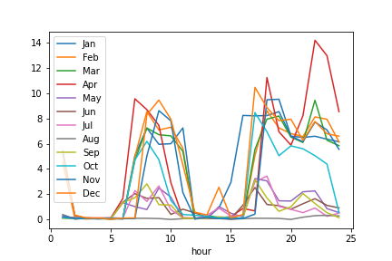
Plotting your data should result in this:
%matplotlib inline
ax1 = piv.plot()
ax1.figure.savefig("day21_months.png")
Expected Result:
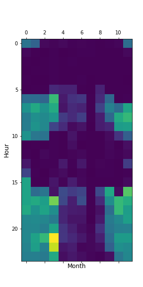
import matplotlib.pyplot as plt

plt.matshow(piv)

plt.xlabel('Month', fontsize = 12)
plt.ylabel('Hour', fontsize = 12)
plt.show()
Expected Result: