.ipynb .pdf

Binder

Contents

Summary of Lessons

1,2: Basics:

# Libraries
from math import exp, sqrt, pi

# Variables
x = 1.75

# Calculations
y = exp(-x**2/2) / sqrt(2*pi)

# Printing
print(f"The PDF of the standard normal distribution at x={x} is {y:.3}")

The PDF of the standard normal distribution at x=1.75 is 0.0863

3. Functions

# Built-in functions

p3 = round(pi, 3)
print(p3, pi)

3.142 3.141592653589793

# Defining a new function
def normal(x, mean=0, stdev=1):
    norm = 1 / ( stdev * sqrt(2*pi) )
    z = (x-mean)/stdev
    PDF = norm * exp(-z**2 / 2)
    return PDF,z

# "calling" a function
y,z = normal(2.75, mean=1)

print(z,y)

1.75 0.08627731882651153

4a. Conditionals

def discuss(zval):
    if -1 <= zval <=1:
        print("This event is quite common!")
    elif -2 <= zval <= 2:
        print("This event not so common!")
    else:
        print("This event is very rare!")
        
discuss(z)

This event not so common!

4b. Iteration

z=-3
while z<=3:
    print("z=", z) 
    discuss(z)
    z = z+0.5

z= -3
This event is very rare!
z= -2.5
This event is very rare!
z= -2.0
This event not so common!
z= -1.5
This event not so common!
z= -1.0
This event is quite common!
z= -0.5
This event is quite common!
z= 0.0
This event is quite common!
z= 0.5
This event is quite common!
z= 1.0
This event is quite common!
z= 1.5
This event not so common!
z= 2.0
This event not so common!
z= 2.5
This event is very rare!
z= 3.0
This event is very rare!

5. Lists and loops

# Creating lists
int_list = list(range(10))

print(int_list)

[0, 1, 2, 3, 4, 5, 6, 7, 8, 9]

# List comprehension
new_list = [n+1 for n in int_list]

print(new_list)

[1, 2, 3, 4, 5, 6, 7, 8, 9, 10]

# for loops
for n in range(11):
    x2 = 0.1*n - 0.5
    print(round(x2,1))

-0.5
-0.4
-0.3
-0.2
-0.1
0.0
0.1
0.2
0.3
0.4
0.5

Example: Numerical Integration

Some functions such as the normal distribution \(\displaystyle y = \frac{1}{\sigma \sqrt{2\pi}} e^{-\frac{1}{2}\left(\frac{x-\mu}{\sigma}\right)^2}\) cannot be integrated analytically (by hand).

We can do this numerically by approximating the area under the curve using finite blocks of width \(\Delta x\) and height \(y\) and adding their area. See the plots in Section 6.

The code below combines the programming building blocks above to approximate the area under (integrate) the normal distribution between two values \(x=a\) and \(x=b\)

from math import exp, sqrt, pi

# Defining the normal distribution function (with standard values as default parameters)
def normal(x, params=None):
    if params==None:
        mean=0 
        stdev=1
    norm = 1 / ( stdev * sqrt(2*pi) )
    z = (x-mean)/stdev
    PDF = norm * exp(-z**2 / 2)
    return PDF

# Define an integration function
def integrate(func, a, b, dx, params=None):
    """Integrates a function named as the first argument 
    between limits a and b with resolution dx
    func(x, params=(p1,p2,...)) must take only one positional argument 
            and possibly optional parameters as a single argument"""
    Area = 0
    x=a
    while x<=b:
        y = func(x, params)
        bar_area = y*dx
        Area += bar_area #adds new bar area to existing area
        x=x+dx
    return Area
        
a = -3; b=3
I = integrate(normal, a, b, 0.1) #true value should be 99.73%
print(f"Estimated probability of being between z={a} and z={b} is {I*100:.3f}%\n") 

# create a list of values for the Cumulative Distribution Function
CDF=[]
PDF=[]
xvals=[]
N = 21 #number of values to estimate
stepsize = (b-a)/(N-1) # N-1 gaps between N values
for i in range(N):
    x = a + i*stepsize
    p = normal(x)
    c = integrate(normal, -10, x, 0.001) # normal(-10) is close to zero
    xvals.append(x)
    PDF.append(p)
    CDF.append(c)
    
print(f"{N} values of the CDF between {a} and {b}:")
for i in range(N):
    print(f"The probability of being below z={xvals[i]:.2} is {CDF[i]:.4f}")

Estimated probability of being between z=-3 and z=3 is 99.728%

21 values of the CDF between -3 and 3:
The probability of being below z=-3.0 is 0.0013
The probability of being below z=-2.7 is 0.0035
The probability of being below z=-2.4 is 0.0082
The probability of being below z=-2.1 is 0.0178
The probability of being below z=-1.8 is 0.0360
The probability of being below z=-1.5 is 0.0669
The probability of being below z=-1.2 is 0.1152
The probability of being below z=-0.9 is 0.1842
The probability of being below z=-0.6 is 0.2744
The probability of being below z=-0.3 is 0.3823
The probability of being below z=0.0 is 0.5002
The probability of being below z=0.3 is 0.6181
The probability of being below z=0.6 is 0.7259
The probability of being below z=0.9 is 0.8161
The probability of being below z=1.2 is 0.8850
The probability of being below z=1.5 is 0.9333
The probability of being below z=1.8 is 0.9641
The probability of being below z=2.1 is 0.9822
The probability of being below z=2.4 is 0.9918
The probability of being below z=2.7 is 0.9965
The probability of being below z=3.0 is 0.9987

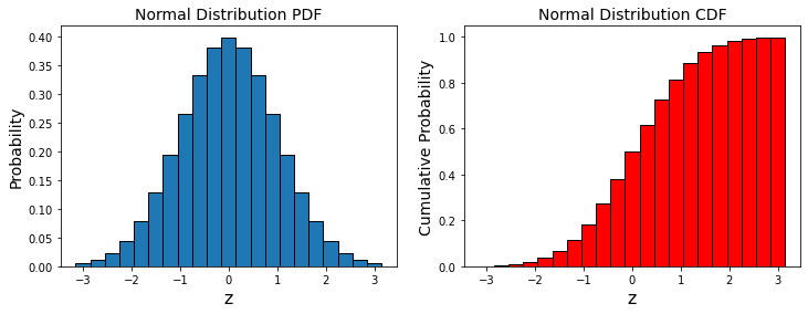
6. Plotting

import matplotlib.pyplot as plt

fig = plt.figure(figsize=(12,4))

ax1 = fig.add_subplot(1,2, 1)
ax1.bar(xvals,PDF, edgecolor="black", width=stepsize)

ax2 = fig.add_subplot(1,2, 2)
ax2.bar(xvals,CDF, color="red", edgecolor="black", width=stepsize)

ax1.set_xlabel("z", size=16)
ax2.set_xlabel("z", size=16)

ax1.set_title("Normal Distribution PDF", size=14)
ax1.set_ylabel("Probability", size=14)
ax2.set_title("Normal Distribution CDF", size=14)
ax2.set_ylabel("Cumulative Probability", size=14)

fig.show()

7+ Manipulating and analysing data

import pandas as pd

# read in external data file
data = pd.read_excel("Files/Case Study Data.xlsx", sheet_name="Data")

cols = ['Project', 'Region', 'Country', 'Type', 'Rating', 
        'Cost.Million.USD','Total.Area.sqm', 'Total.Delivered.kWh']
data[cols]

	Project	Region	Country	Type	Rating	Cost.Million.USD	Total.Area.sqm	Total.Delivered.kWh
0	Manitoba Hydro Place	Americas	Canada	Commercial	LEED-Platinum	269.660000	65000.000000	7.280000e+06
1	Child Development Centre	Americas	Canada	University	LEED-Platinum	22.310000	11612.140575	1.817300e+06
2	FIPKE Centre for Innovative Research	Americas	Canada	University	Green-Globe-5	30.555000	6323.794118	2.365099e+06
3	Transoceanica	Americas	Chile	Commercial	LEED-Gold	20.924644	13959.068901	7.496020e+05
4	The Cooper Union	Americas	United States	University	LEED-Platinum	112.000000	16255.124535	8.745257e+06
5	Biodesign Institute B	Americas	United States	University	LEED-Platinum	78.500000	27184.466019	2.520000e+07
6	DELL Children's Medical Center of Central Texas	Americas	United States	Hospital	LEED-Platinum	137.000000	43948.234956	3.990500e+07
7	Kroon Hall	Americas	United States	University	LEED-Platinum	33.500000	6205.254065	6.105970e+05
8	Newark Center at Ohlone College	Americas	United States	University	LEED-Platinum	58.000000	12806.321244	1.235810e+06
9	Tahoe Center for Environmental Sciences	Americas	United States	University	LEED-Platinum	25.000000	4374.310680	4.505540e+05
10	Center for Health and Healing, Oregon	Americas	United States	University	LEED-Platinum	145.400000	38143.178709	1.784338e+07
11	NREL Research Support Facility 1	Americas	United States	University	LEED-Platinum	91.400000	33457.000000	3.713727e+06
12	Twelve West	Americas	United States	Commercial	LEED-Platinum	138.000000	39747.000000	5.476264e+06
13	2000 Tower Oaks Blvd	Americas	United States	Commercial	LEED-Platinum	63.600000	18619.361936	3.385000e+06
14	Regent's Hall	Americas	United States	University	LEED-Platinum	63.000000	17859.989362	3.357678e+06
15	Great River Energy	Americas	United States	Commercial	LEED-Platinum	65.000000	15434.070000	3.086814e+06
16	Lewis & Clark State Office building	Americas	United States	Commercial	LEED-Platinum	18.100000	11324.251203	2.513984e+06
17	Johnson Controls Campus	Americas	United States	Commercial	LEED-Platinum	73.000000	28745.989412	7.330227e+06
18	Genzyme Center	Americas	United States	Commercial	LEED-Platinum	140.000000	32021.614035	9.126160e+06
19	CSOB	Europe	Czech Republic	Commercial	LEED-Gold	107.000000	82365.580435	1.515527e+07
20	Lintulahti	Europe	Finland	Commercial	LEED-Platinum	29.500000	12885.708920	2.744656e+06
21	EMGP 270	Europe	France	Commercial	HQE-Office	24.900000	9983.377193	2.276210e+06
22	Paul Wunderlich-Haus	Europe	Germany	Public Sector	DNGB-Gold	32.265000	22000.000000	1.056000e+06
23	Federal Environmental Agency	Europe	Germany	Public Sector	DNGB-Gold	91.800000	41000.000000	3.513700e+06
24	Heinrich Boll Foundation	Europe	Germany	Public Sector	DNGB-Gold	16.875000	6964.509202	6.811290e+05
25	Solon Corporate HQ	Europe	Germany	Commercial	DNGB-Gold	63.450000	33451.000000	3.646159e+06
26	Thyssenkrupp Q1	Europe	Germany	Commercial	DNGB-Gold	116.000000	29000.000000	4.350000e+06
27	SAP	Europe	Ireland	Commercial	NaN	18.000000	6000.000000	1.009421e+06
28	Hagaporten 3	Europe	Sweden	Commercial	Miljobyggnad-Gold	130.000000	30000.000000	4.050000e+06
29	Eawag Forum Chriesbach	Europe	Switzerland	Commercial	NaN	32.745000	8533.000000	4.197950e+05
30	Daniel Swarovski Corp	Europe	Switzerland	Commercial	NaN	57.000000	12627.187079	9.382000e+05
31	TNT Express HQ	Europe	The Netherlands	Commercial	LEED-Platinum	NaN	17250.000000	1.966500e+06
32	3 Assembly Square	Europe	United Kingdom	Commercial	BREEAM-Excellent	19.500000	6106.699387	9.953920e+05
33	Suttie Centre	Europe	United Kingdom	University	BREEAM-Excellent	22.356000	6500.000000	1.098500e+06
34	2 Victoria Avenue	Asia-Pacific	Australia	Commercial	Green-Star-Office-6	NaN	7185.000000	7.008530e+05
35	Workplace6	Asia-Pacific	Australia	Commercial+Retail	Green-Star-Office-6	52.080000	18000.000000	2.052000e+06
36	One Shelley Street	Asia-Pacific	Australia	Commercial+Retail	Green-Star-Office-6	NaN	33000.000000	4.929499e+06
37	Council House 2	Asia-Pacific	Australia	Public Sector	Green-Star-Office-6	71.740200	12536.000000	2.295816e+06
38	The Gague	Asia-Pacific	Australia	Commercial+Retail	Green-Star-Office-6	NaN	10366.000000	2.467108e+06
39	Vanke Center	Asia-Pacific	China	Commercial	LEED-Platinum	NaN	14239.000000	1.980000e+06
40	Suzlon One Earth	Asia-Pacific	India	Commercial	LEED-Platinum	NaN	75809.000000	4.472731e+06
41	Keio University 4th Building Hiyoshi Campus	Asia-Pacific	Japan	University	CASBEE-S	NaN	18399.000000	2.907042e+06
42	Epson Innovation Center	Asia-Pacific	Japan	Commercial	CASBEE-S	NaN	53372.000000	8.966496e+06
43	Honda Wako	Asia-Pacific	Japan	Commercial	CASBEE-S	NaN	52112.714286	1.203804e+07
44	Nissan Global HQ	Asia-Pacific	Japan	Commercial	CASBEE-S	NaN	78500.000000	2.457050e+07
45	Kansai Electric Power HQ	Asia-Pacific	Japan	Commercial	CASBEE-S	NaN	60000.000000	2.028000e+07
46	Zero Energy Building	Asia-Pacific	Singapore	Public Sector	Green-Mark-Platinum	8.800000	4500.000000	1.831500e+05
47	School of Art, Design, Media at NTU	Asia-Pacific	Singapore	University	Green-Mark-Platinum	28.800000	19975.000000	2.692630e+06
48	Magic School of Green Technology	Asia-Pacific	Taiwan	University	LEED-Platinum	6.000000	3055.000000	1.235136e+05

# manipulating data
cost_per_square_m = data["Cost.Million.USD"] / data["Total.Area.sqm"]
data["cost_per_square_m"] = cost_per_square_m

# interactive plotting (hover mouse over points)
import plotly.express as px

fig = px.scatter(data, x="Delivered.Intensity.KWh.sqm.y", y="cost_per_square_m", 
                 hover_data=["Project", "Rating"])
fig.update_traces(marker=dict(size=12))

Installing and Running Python on Your Own Computer