Machine Learning 2
Regression
Introduction
In this lab you will practice solving regression problems. You will practice parametric regression, mainly based on synthetically generated data. Next, you will experiment with regularization, a method to control the regression coefficients. Lastly, you will look at non-parametric regression models (such as neural networks), feature ranking, hyperparameter optimization and testing.
Regression
As opposed to classification, in regression we’re not predicting one element in a finite (and rather small) set of options (e.g., the class index from a set of three possible plant species), but rather an element in a (theoretically) infinite set of possibilities (e.g., the temperature data from a sensor, voice recordings, stock market prices).
In this case, we will use a specialized Matlab app called the Regression Learner. If you did not already, it is recommended that you go through the previous lab on classification, which contains an introduction to the Classification Learner Matlab app. This would give a useful introduction to the Regression Learner app used in this lab script.
Parametric Regression
In parametric regression, we assume we know the model describing the data, and the purpose is to fit the parameters. We will go through linear and quadratic regression.
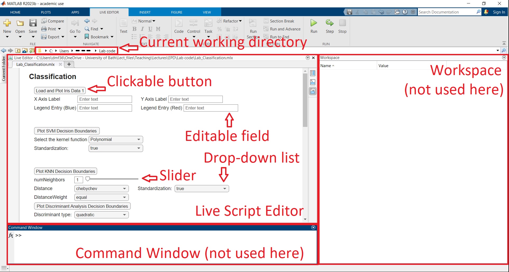
We will first load the first regression dataset, which consists of noisy points along a curve, but with outliers. Open the live Matlab script Lab_Regression.mlx. One of the most common Matlab errors is that the current working directory is not set to the folder immediately above the Matlab script being executed (in this case Lab_Regression.mlx). Locate the working directory based on the image below and ensure it’s set to the corresponding folder.
Click on ‘Load & Plot Regression Data 1’.
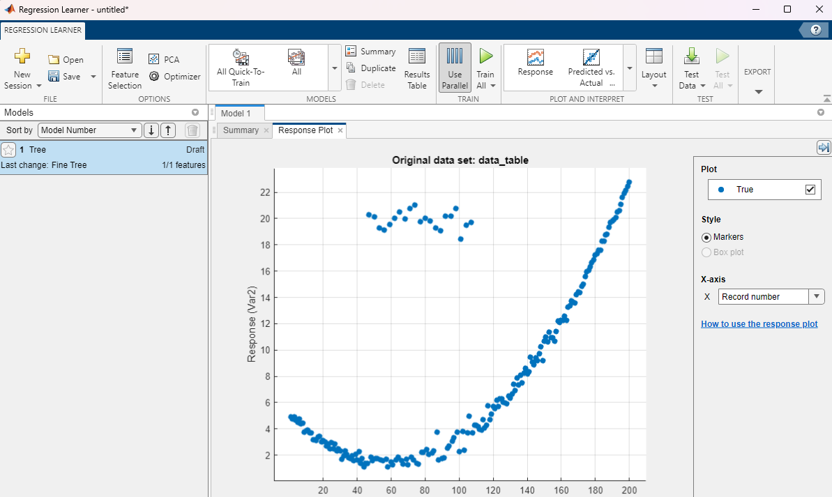
Let us open the Regression Learner app. In the APPS tab at the top of the Matlab window, click on the down arrow to expand the list of apps. Select the Regression Learner. Click on the yellow cross to open a new session by selecting data from the workspace. In the New Session window, ensure that data_table is selected as Data Set Variable. In the Response section, the “From data set variable” option should be ticked, and the Var2 variable selected. Click on “Start Session”. You should see something like below:
Expand the MODELS section at the top by clicking on the down arrow. Select a Linear model. This adds a new draft model instance. To avoid any confusion, right-click on the default model instance “Tree” and click delete as below (make sure to not delete the Linear model). Train your model. The predicted values show up in the same plot.
Recall (or search) the definition of the Root Mean Squared Error (RMSE). Assuming the data points are voltage measurements is mV, what will be the measurement unit for RMSE?
Duplicate the linear model. In the Summary of the new draft, under Model Hyperparameters, select Quadratic terms and train the model again.
What can you say about the two errors, comparatively, in terms of RMSE?
Visually, why do you think that the last model is not performing ideally? After all, the data looks to follow a quadratic trend!
Duplicate the model again. This time, in addition to quadratic terms, switch the Robust option to On. Train the model.
How is the performance compared to the previous models in terms of RMSE?
What about visually, when looking at the predictions?
Can we state that the RMSE is always the best evaluation of performance?
What do you think the robust option is doing?
Regularization
Regularization has the main purpose to shrink the regression coefficients to produce similar models when the training data changes.
In the live Matlab script, click on ‘Load & Plot Regression Data 2’. This loads a dataset of noisy linear observations. Then open the Regression Learner from the APPS section at the top of the Matlab window. Start a new session with data from the workspace (you may choose if you want to save the previous session). For the Data Set Variable, select data_table2. For the Response, ensure you ticked the “From data set variable” option, and selected variable y. In the validation section, as before, we will leave it as the default option of 5-fold cross-validation. As opposed to the previous examples, here we will include a testing dataset to evaluate the generalizing ability of the model. In the Test section, tick “Set aside a test data set”, and set the “Percent set aside” as $20\%$. This means that $20\%$ of the data will be not be “seen” by the model during training, and will be used at the end to see how the model performs on entirely new data.
Click “Start Session”. In the MODELS section at the top, use the down arrow to select a Linear model and an Efficient Linear Least Squares model. As before, delete the default tree model. The linear model simply performs a linear fit with no regularizaiton. For the Efficient Linear Least Squares model, under regularization, pick Ridge. Duplicate the model, and change the regularization to Lasso for the new model.
Train all the models. Select the Linear Regression model, and open the Response Plot.
Why are the predicted values not on an exact straight line? Remember that the predicion output is not corrupted by noise. (Hint: think about the validation method used)
Which model leads to the lowest Validation RMSE values? How can you explain this?
Recall that in the beginning of this example we have set aside $20\%$ of the data for testing. This portion of the data, which was not used for cross-validation, will generate a different RMSE performance.
At the top of the Regression Learner window, select the TEST section. Locate the green triangle at the top labelled “Test All” and click on it. Notice that the RMSEs shown for each model are now Test RMSEs.
What can you say about the performance of the models on the testing data?
Pick a new Efficient Linear Least Squares model (or duplicate an old one), set the Regularization to Ridge, the Regularization strength (Lambda) to Manual, and increase it significantly. Duplicate this model a couple of times and keep increasing the regularization parameter until it reaches large values ($>1$).
What do you notice about the RMSEs and the Response Plots?
Trying to generalise this, how is the model responding to the input data for very large regularization values?
Non-Parametric Regression
In most practical applications, we measure a number of input variables and try to predict an output variable without knowing what the underlying model is.
We will look at an example dataset where we try to predict a car’s fuel economy based on $14$ different features. Click on “Load Regression Data 3” in the live script, and open the Regression Learner if you haven’t already. Click on the yellow cross (under the LEARN tab) to start a new session. For the Data Set Variable, you should have “data_table3” selected. The Response should be toggled to “From data set variable”, and chosen as FuelEcon. In the Predictors section, you should have $14$ features selected. Inspect those features to get a basic understanding of the data.
In the Cross-Validation section leave the default 5-fold cross-validation. In the Testing section choose to reserve $20\%$ of the data for testing.
Start the session. On the right-hand side, you should be able to see the response plot for the case of the default Fine Tree model. In the X-axis currently “Record number” is selected. The ML models are not using this, as this is not one of the features, and it’s only used for display purposes. If you expand the drop-down list, you will have the option to choose one the $14$ features to be displayed on the X-axis. Keep changing the features to see how the FuelEcon is affected by each of them. Notice that some of the features are categorical (Car_Truck, AC), whereas others are non-categorical, changing continuously (Weight, RatedHP).
Feature Ranking
Clearly, there is a link between all these features and the fuel economy. However, we don’t know what the underlying model is. Moreover, even if the model were known, one single feature on its own may be a bad predictor.
Among the $14$ features available, select the features that you think are the best predictors of fuel economy, and which features are the worst predictors. Write down the results.
You should have noticed that none of the features suggest there is a one-to-one model between that feature and fuel economy, allowing the prediction from that feature alone.
What you have attempted in the last step is formally known as “feature selection”. Let’s see if any of your selected features are also idenfied as important/unimportant by the regression learner.
At the top of the Regression Learner window, in the LEARN section, click on the Feature Selection button under the OPTIONS category, as below:
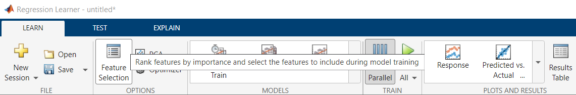
There are different ranking algorithms that may lead to different results. Currently, “None” is selected. Switch to “F Test” and inspect the result. A high F Test score means that feature is considered particularly important. Similarly, have a look at the ranking decided via the “MRMR” algorithm.
How are the features you identified in the previous step ranked by the two algorithms?
What are the features identified to be most relevant by both algorithms?
Regression with Neural Networks
In this example, we will use neural networks to model and predict. The massive advantage of neural networks is that they do not need to know the underlying model. You can give the network different features and it can figure out by itself which ones are more important than others and “learn” the underlying models between those features and the output. However, the final result depends a lot on the settings of the neural network, also called hyperparameters. There are a lot of hyperparameters that can be tuned for a network, but we will limit this study to the following:
- Number of fully connected layers
- Size of each layer (number of neurons)
- Activation function (ReLU, Sigmoid, Tanh)
- Regularization strength (parameter $\lambda$ controls regularization, i.e., “shrinking” the network weights, see the previous section on regularization)
- Data standardization (Yes/No)
From the MODELS section at the top of the window, add $3$ draft models: a Narrow, a Medium and a Wide Neural Nework. These are $1$-layered neural networks of various sizes, which can be viewed in the Summary section after selecting each draft model. Train the three models, and inspect the validation RMSEs and the response plots. Change the feature on the X-axis for each model, to see how well the model captures the link between that feature and the fuel economy.
Note that all these models are using a ReLU activation function, which is rather simple. Let’s duplicate all three models, and select the Sigmoid activation function for each. Train these three new models.
Leave the X-axis set on “Record number”. Untick the “Predicted” box, to show only the True values, as shown below:
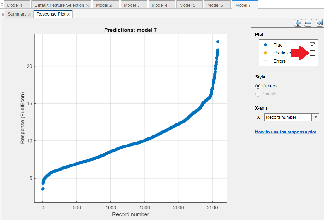
By ticking and unticking the “Predicted” box, notice how the predicted values are very spread out around the true values for all models.
Can we conclude that all neural networks are struggling to fit the relatively simple blue nonlinear monotonic curve? (Hint: Remember what we are trying to achieve)
Notice that even though we have six models, there are many more first layer sizes that were not evaluated yet. Moreover, we did not change the iteration limit, regularization, or if the data is standardized.
Keep duplicating the three types of networks (Narrow, Medium, Wide), and iteratively adjust the hyperparameters in the Summary section. Train the new models. What’s the smallest RMSE you can achieve? How does it compare to your colleagues’ result? Write down the result.
Hyperparameter Optimization
Before moving to this section, make sure the previous tasks were achieved, and you have some time remaining in the lab session. This section may take a while, and cancelling the optimization before it is completed may cause Matlab to freeze.
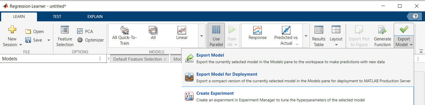
Clearly, trying out all combinations of hyperparameters by hand is not feasible. Let us fit these parameters automatically. Select the model with the lowest validation RMSE. At the top of the Regression Learner window, select the LEARN section. In the top right, you will see a button with a green tick labelled “Export Model”. Click on the lower half of this button to expand a drop-down list with three options, as below:
Click on “Create Experiment”. You will be prompted to choose the names of a .mat file and a .m file. We won’t deal with these files directly. Leave the default names, and just click on “Create Experiment”. Click on “Ok” to confirm starting a New Project. On the next window, leave the default name and path, and click Save.
This will open several windows, but we will only deal with the Experiment Manager Window, which should look as below:
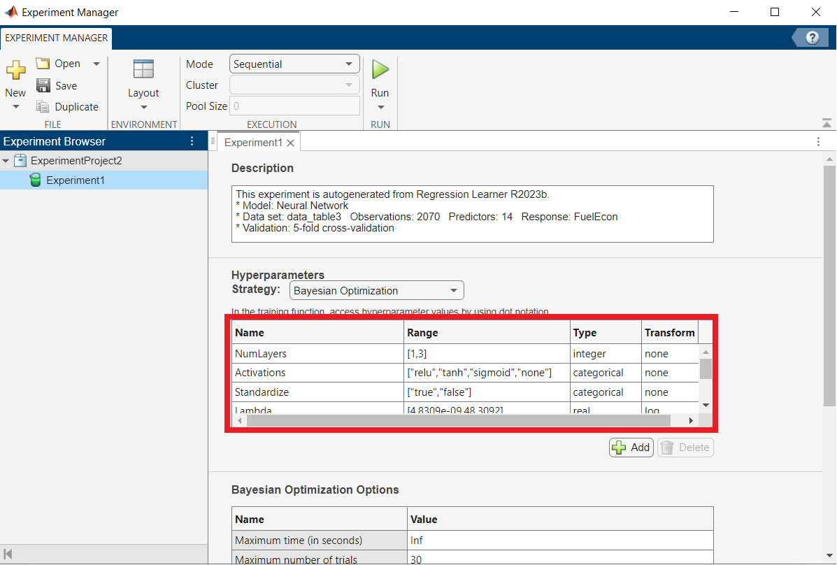
In the highlighted section, you can see the ranges in which the optimization algorithm will search for each parameter.
What are the potential problems of choosing very wide ranges, including options with very large layer sizes or numbers of layers? At least two should come to mind.
In the highlighted section above, scroll down to the hyperparameter called “Layer3_Size”. Change the range for both Layer2_Size and Layer3_Size from $[1,100]$ to $[1,2]$. This is to speed up the optimization. Then change Layer1_Size to $[1,300]$.
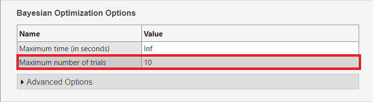
We leave the Strategy set to Bayesian Optimization. In the Bayesian Optimization Options section, change the “Maximum number of trials” from $30$ to $10$ as below:
This is again to speed up the optimization. At the bottom of the Experiment Manager window, in the Metrics section, check that we are minimizing ValidationRMSE.
At the top of the Experiment Manager, click on the green triangle labelled “Run” to start the hyperparameter optimization.
After the optimization is finished, a new tab will open under the “Run” button, entitled something like “Experiment1 | Result1”. To run the experiment again, you will need to first switch back to the previous tab “Experiment1” before clicking on “Run” again. Feel free to run a few more sessions in this way (depending on how long it takes). Hint: asking the optimizer to search among larger sizes for layer $1$ tends to lead to better results (e.g., setting a higher minimum size by adjusting Layer1_size).
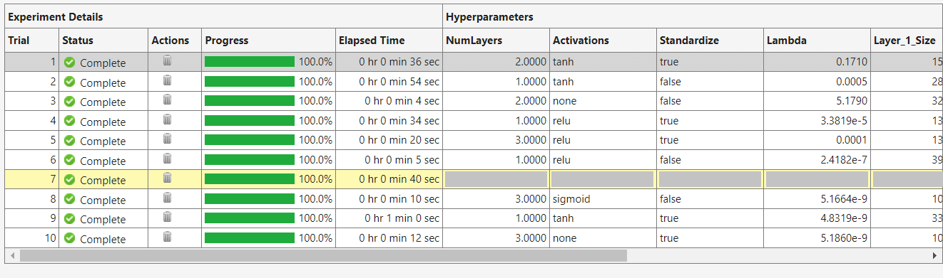
Locate the best performing model from all experiments, which is highlighted in the bottom part of the Experiment Manager window for each experiment as shown below:
What is the lowest validation RMSE you could achieve?
Try to get a lower RMSE than the best one you achieved in the Regression Learner. Once this is done, let’s transfer those hyperparameters in the Regression Learner. Duplicate any of the neural network models in the Regression Learner. In the Summary section of that model, copy the all the hyperparameters of the best performing model from the Experiment Manager window (Num_Layers, Activations etc.). Train the model in the Regression Learner. If this was done correctly, the validation RMSE should be close to the RMSE in the Experiment Manager, and lower that the RMSE achieved by all other models in the Regression Learner.
Testing
We trained a number of models, but how well do they generalize on an “unseen” dataset? Recall that in the beginning of the session, we allocated $20\%$ of the data for testing, which was not used during training.
At the top of the Regression Learner window, click on TEST to evaluate the results on the testing “unseen” dataset. Click on the green triangle labelled “Test All”.
Which of the models achieved the smallest RMSE on the testing data?
How well do the best performing models generalize? In other words, are the best performing models on the training data also competitive on the testing data?
Unsupervised Learning
An important unsupervised learning method is the Principal Component Analysis (PCA). PCA decreases the dimensionality of the data, allowing to vizualize the data easier, and also remove the less important features.
Going back to the Regression Learner app, duplicate your best performing model. In the Summary of that model, tick the box as below to Enable PCA:
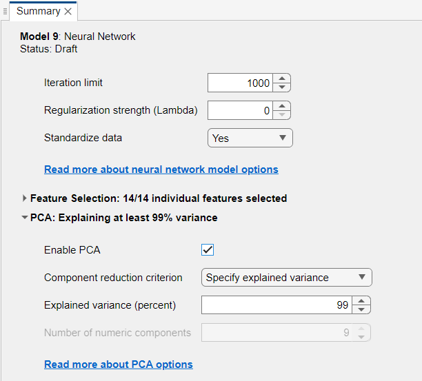
Reducing the explained variance from $100\%$ will also reduce the numbers of features in the model. Duplicate the model several times, with an explained variance between $95\%$ and $100\%$ (you can also try to go lower).
How is the performance affected?
Which of the models would you choose, in order to have a compromise between the performance and simplicity?
Further Work
You can test the ML models above with different datasets. There are a lot of datasets available online. An example is the default ML datasets on the Mathworks website: https://uk.mathworks.com/help/stats/sample-data-sets.html
To evaluate a new dataset, you can ignore the Live Editor window and type in the Command Window (locate it using the first figure in this lab script) the commands to load the dataset into the memory. For example, for the hald.mat dataset, type the following in the Command Window and then press Enter:
1
2
clear all;
load hald.mat;
If the dataset is in the section “Data Sets Available with Specific Examples” from the link above, such as the arrythmia.mat dataset, the data can be loaded by typing the following in the Command Window and then pressing Enter:
1
2
3
clear all;
openExample("arrhythmia.mat");
load arrhythmia.mat;
After this, start a new session with the Regression Learner, and load the corresponding variables in the app to train models as above. Of course, you need to first understand the dataset, and make sure it is compatible with the problem you are trying to solve. For this, you can look at the variables in the Workspace (see the first figure in this lab script), and double click on each one to see their contents. Many of the datasets contain a variable called “Description”, which provides further information.
A full documentation of the Statistics and Machine Learning Matlab Toolbox can be found at: https://uk.mathworks.com/help/stats/index.html. This includes the documentation of all machine learning models supported by the toolbox (including the ones discussed in this lab) and also all functionalities of the Regression Learner app, located in the Regression section of the documentation website.