Machine Learning 1

Classification

Introduction

In this lab you will practice solving classification problems. The examples will mainly focus on Fisher’s Iris dataset, but you will learn how to process your datasets of choice at the end, in the Further Work section. The examples will be run in Matlab, either in the live script editor, or in various Matlab apps.

Setting up the Matlab Environment

Download all files in the same folder named “Lab code” (or any other name of your choice), then double click on Lab_Classification.mlx. A Matlab window should open looking something like this:

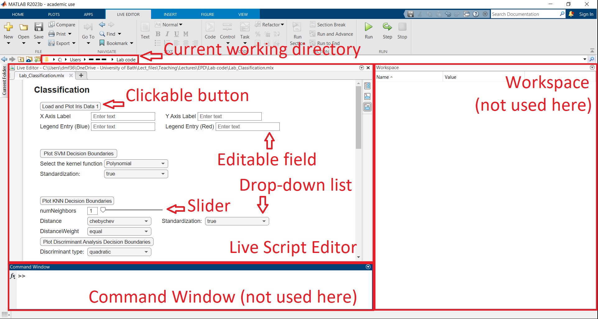
The sections such as Workspace, Editor etc. may be positioned differently in your case by default. However, we only need the Live Script Editor for most of the lab. In any case, one of the most common Matlab error is that the current working directory is not set to the folder immediately above the Matlab script being executed (in this case Lab_Classification.mlx). If you followed the instructions, this should not happen, but it’s worth double checking that this is true.

Open the live Matlab script Lab_Classification.mlx. Ensure that the “Hide Code” visualization option is selected on the right-hand side of the Live Editor:

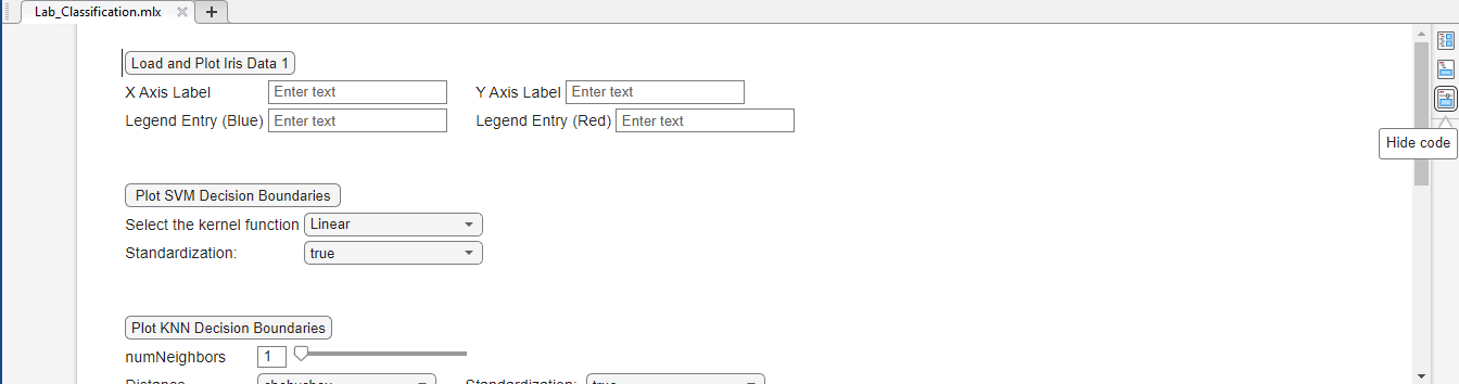
When running the script sometimes it may switch from the “Hide Code” mode if there are errors, and start showing code. You should not edit code at this stage, so please click again on “Hide Code” if this happens.

Classification Models

Fisher’s Iris Dataset

In this lab, we will go through a famous dataset used for classification, known as Fisher’s Iris dataset. This dataset consists of Iris flowers and records features of three Iris species: Iris setosa, Iris virginica and Iris versicolor. The corresponding features of each flower are: sepal length, sepal width, petal length and petal width.

Click on ‘Load & Plot Iris Data 1’. This loads 2 features corresponding to Iris virginica and Iris versicolor. Using fewer features and examples allows for a clearer 2D visualisation. Moreover, this button also allows you to visualise the dataset. We know that one datapoint in this dataset corresponds to Iris versicolor and has a petal length of 4.1 cm and petal width of 1.3 cm.

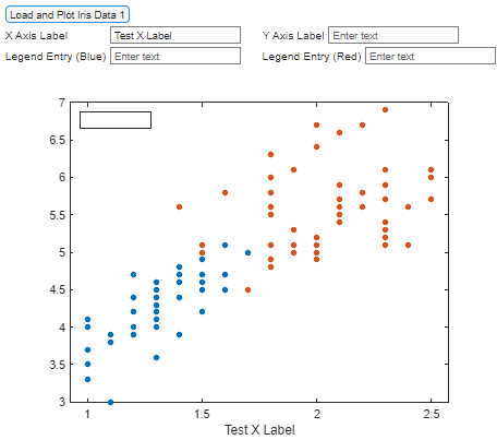
Based on the information above, label correctly the X-axis, Y-axis and legend.

For example, when we type in the first box ‘Test X Label’ and click outside the box, we should see something like this:

Support Vector Machines (SVMs)

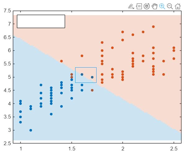
Let’s now visualize what the predicions of various ML models look like for this dataset. To train an SVM click on ‘Plot SVM Decision Boundaries’. This allows you to see what prediction the SVM would make for new datapoints, when trained on Iris Data 1.

Knowing that there are a total of $100$ datapoints (corresponding to both classes), can you work out the training accuracy? Write down the results.

If needed, you can zoom in by first clicking on the figure to select it, then clicking on the magnifier as below:

Try different kernel functions and standardisations.

What is the lowest training error you can achieve? Write down the results.

What conclusion can you reach on using linear versus nonlinear kernel functions?

K-Nearest Neighbors (KNNs)

Let’s repeat the process for a KNN classifier. Here, we can select the number of neighbours, the type of distance used, the standardisation, and distance weight (i.e., what distance metric to use for prediction).

Can you get $100\%$ accuracy? If not, what is the highest you can get, and for what parameter choices? Write down the results.

What do you think is the main issue to look out for when getting a $100\%$ training accuracy?

When comparing the decision boundary for cityblock and euclidian distances, what do you notice regarding the decision boundary? Can this be explained via the definition of the two distances?

Discriminant Analysis

Lastly, let’s have a look at the decision boundaries of the discriminant analysis with various discriminant types.

Plot the boundaries for all $6$ possible types and compare the results.

Trying Out Various Datasets

Looking back at your X and Y labels, notice that we only selected $2$ features out of the possible $4$. Two further datasets were created, called Data $2$ and Data $3$, respectively. They both have a feature in common with Data $1$. Additionally, they are characterised by the sepal length.

Click on “Load & Plot Iris Data 2” and “Load & Plot Iris Data 3”.

Just by investigating the plotted datasets and looking at the X and Y coordinates of the points, can you correctly label the X and Y axes of Data $2$ and Data $3$?

Training SVM, KNN and Discriminant Analysis on New Datasets

Repeat the processes before to plot and tune the decision boundaries of the three ML models. Make sure to click on the “Load & Plot Iris Data” corresponding to the correct dataset before plotting the decision boundaries.

Write down the results of the new optimal parameters achieved for these new datasets.

Do you notice any similarities between datasets?

Training on Multidimensional Datasets

You noticed we could view the same dataset in separate ways by extracting a different pair of features. This was mostly for illustration purposes, i.e., $3$ dimensional patterns of the data points are difficult to see on a flat screen. Clearly, we cannot view more than $3$ dimensions. However, this does not stop us from processing them, because we can simply extend the 2D linear algebra to arbitrarily large dimensions.

Let us now process the full 4-dimensional Iris dataset. Click on “Load Full Iris Data”. This loads all four features (sepal length, sepal width, petal length and petal width), and also all three flower species (Iris setosa, Iris virginica and Iris versicolor).

What is the total number of dimensions and decision boundaries we would need to generate figures similar to the ones generated with the previous datasets?

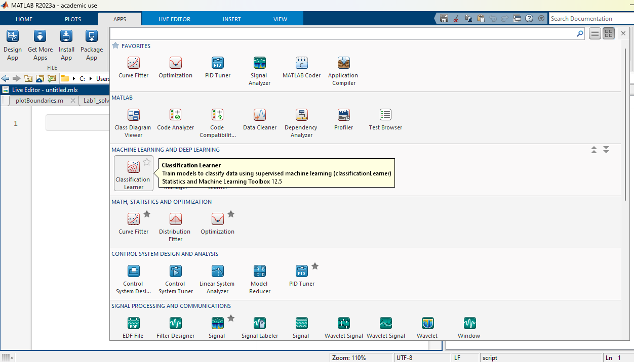
To process this high dimensional data we will use an existing Matlab app called “Classification Learner”. Click on “Apps” at the top of the matlab screen, and select “Classification Learner” as shown below:

Here we use the full Fisher’s Iris dataset previously loaded in Matlab’s memory (if you closed Matlab, make sure you open again the live editor and click on “Load Full Iris Data”).

In the Classification Learner window, click on the yellow cross to start a new session by selecting data from the workspace. When prompted to select the Data Set Variable, choose matrix X, containing the features of the dataset. For the Response, tick the “From workspace” option, then confirm that variable y is selected, containing the class name corresponding to each example with features in X:

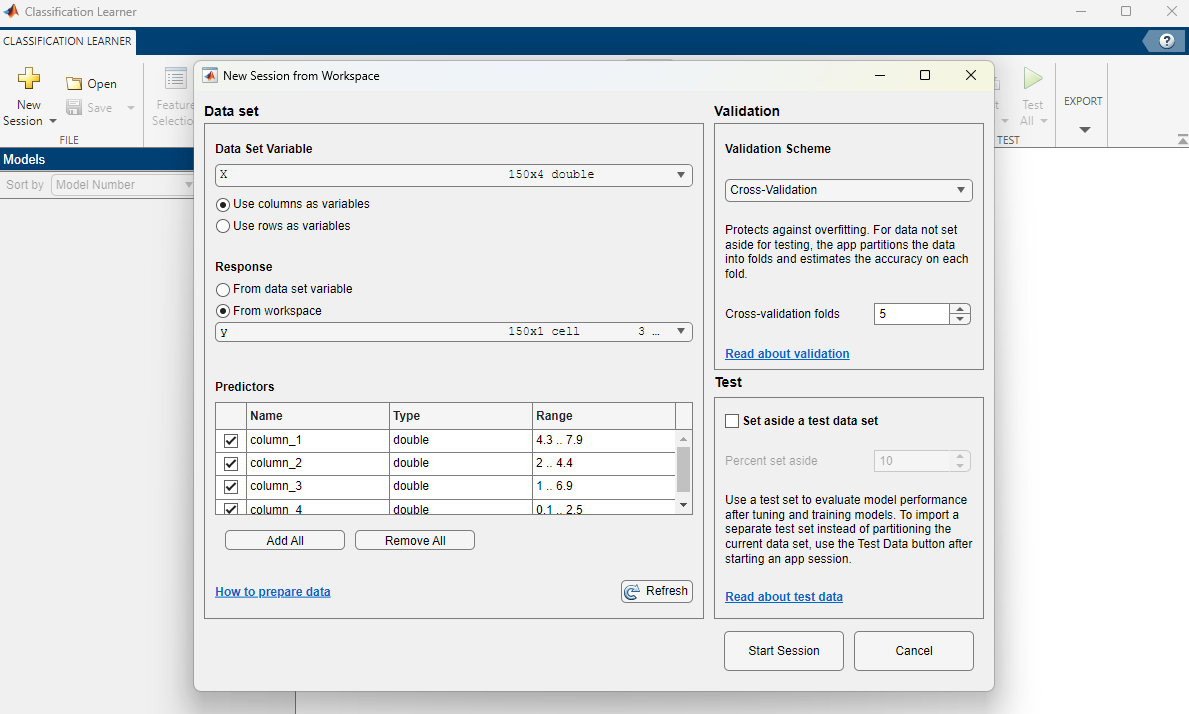
We will not use a testing dataset in this case. Click on “Start Session”. You should see something like below:

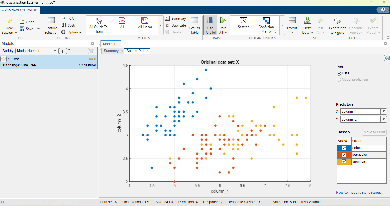
A scatter plot shows, as in the previous live editor examples, two features of the input dataset. In the right-hand side of the screen, under “Predictors”, you can use the drop-down lists to change which two features of the input will be used for the scatter plot. Moreover, under “Classes”, you can tick and untick to select the flower classes shown in the plot.

By adjusting the “Predictors” and “Classes” sections, achieve the same scatter plot as previously in the live editor, under “Load and Plot Iris Data 1”.

With all $3$ classes displayed, investigate which of the $4$ features allow the easiest discrimination between flower species setosa and versicolor?

Support Vector Machines

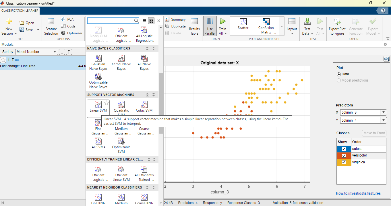
Let us now train an SVM model. From the “MODELS” section at the top of the page, click on the arrow to show all models available, then scroll down and select the linear SVM as below:

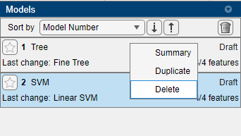
This adds a new draft model instance. To avoid any confusion, right-click on the default model instance “Tree” and click delete as below (make sure to not delete the SVM):

We are prompted to choose some model hyperparameters for the SVM. Let’s keep the kernel function as linear, and the multiclass method as “One-vs-One”. Click on the green triangle at the top of the page, under the “TRAIN” section, to train all draft models. Notice the time taken for training. The resulted accuracy will be displayed on the right-hand side, next to the model instance. The confusion matrix shows the misclassified examples in each class.

Which classes are most often misclassified by this SVM instance?

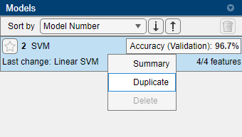
We now want to train another SVM model with different hyperparameters. Rather than looking for the model again, we can right-click on the model instance on the right, and select “Duplicate”:

This creates a new draft model. Change the multiclass method from “One-vs-One” to “One-vs-All”. Train all draft models (the previous SVM model is no longer a draft after training, so won’t be retrained). Notice the time taken for training, and the new accuracy.

Which of the two models was faster to train?

Work out how many different binary classifiers are trained for the “One-vs-One” and “One-vs-All” cases, respectively.

Note that in this case the higher performance of “One-vs-All” is also because the classes are balanced (approximately the same number of examples in each class).

K-Nearest Neighbors

From the “MODELS” section at the top, select “Fine KNN”. Create and train a few KNN models with different numbers of neighbors and distance metrics.

What is the best accuracy you can achieve?

Check the best hyperparameters identified for the datasets with two features in the live editor.

How do they perform on the 4-feature dataset when trained with the Classification Learner app?

How can the difference in performance be explained?

Discriminant Analysis

Similarly, try training a Linear Discriminant and Quadratic Discriminant model in the Classification Learner.

Logistic Regression

In the list of models, select Efficient Logistic Regression. Test out various values of the solver and multiclass coding.

What is the best accuracy that can be achieved with all models? (SVM, KNN, Linear/Quadratic Discriminant)

Based on the confusion matrices, which were the classes that were most often confused by all classifiers?

Neural Networks

To select a neural network classifier, scroll to the bottom of the list of models, and select a Narrow Neural Network, Medium Neural Network, Wide Neural Network, Bilayered Neural Network and Trilayered Neural Network. Train all models on the dataset.

What is the best accuracy achieved?

Rather than hand-picking all hyperparameters (such as number of layers, size of each layer), we can let the Classification Learner optimize this for us. Select the last item in the list of models, called “Optimizable Neural Network”. Note that here all hyperparameters are by default optimized based on the dataset. One can untick the box corresponding to any given hyperparameter to freeze it to a given value and only optimize the remaining ones. For now, leave all boxes ticked apart from the third layer, so that we optimize all hyperparameters.

Recall how 5-fold cross-validation works. How many datapoints are used at any point to evaluate the parameters and hyperparameters, respectively?

Train the Optimizable Neural Network. Notice that a new window appears called “Minimum Classification Error Plot”. This window shows, in real time, how the minimum error changes. At the same time, on the right-hand side, you can see the hyperparameters being tested at any one time, changing from one iteration to the next.

What is the highest accuracy and best choice of hyperparameters? Write down the results.

Unsupervised Learning

So far, we considered cases where the class labels are known, and we are trying to predict them as accurately as possible. However, in many situations, the labels would not be known. Training ML models to perform tasks on unlabelled data is known as unsupervised learning. We will go through two important examples below.

Clustering

Imagine, in the case of Fisher’s Iris dataset considered previously, that somebody measures the sepal length, sepal width, petal length and petal width of $150$ unknown flowers, and has no knowledge of the species. Moreover, they are likely to not know even how many different species are amongst these flowers. This problem may seem much more difficult, but it is still possible to tackle using a process called “Clustering”.

In Lab_Classification.mlx, scroll to the section called “Clustering”, and click on “Load and Plot Iris Data 3 (Clustering)”. Note that this is the same as Data $3$ that we used for classification. However, now all points have the same colour, and we don’t know which class they belong to during training.

One of the basic methods for clustering is k-means clustering, which aims to partition the observations into k clusters, in which each observation belongs to the cluster with the nearest mean. The term “nearest” requires defining a distance metric. We will use three distance metrics: squared Euclidian (sqeuclidian), cityblock and cosine. As the name suggests, in k-means clustering we need to set the number of clusters k.

Before moving to the next section “Classification without class labels, but validation with class labels”, ensure the last button you clicked on was “Load and Plot Iris Data 3 (Clustering)”, otherwise you will get an error. Set different numbers of clusters and distance metrics in the next section, and find the combination that yields the smallest classification error.

How does this classification error compare to the error achieved previously for KNN, Discriminant Analysis and SVM on the same dataset Data $3$?

How can you explain this?

You may have noticed that, in order to calculate the classification error, we need to know the labels. However, this is not used for training, but rather for validation, i.e., choosing the hyperparameter k. For most clustering problems we wouldn’t even be able to find the classification error, because the labels would be unknown. In this case, we can use an evaluation metric called the “silhouette value”.

The silhouette value is a measure of how similar an object is to its own cluster (cohesion) compared to other clusters (separation). In the section entitled “No knowledge of the labels either for training or validation”, you can search for the correct number of clusters by evaluating the silhouette value. Select the minimum and maximum numbers of clusters. Change the distance metric and find the number of clusters and metric with the highest silhouette value.

What is the largest silhouette value you could achieve, and for what number of clusters and distance metric?

Let’s perform clustering, in a more automatic way, using the full Fisher’s Iris dataset (rather than Data $3$ with just two species and two features). Scroll up and click on “Load Full Iris Data” right above “Clustering”. Then scroll down and locate the “Cluster Data” task:

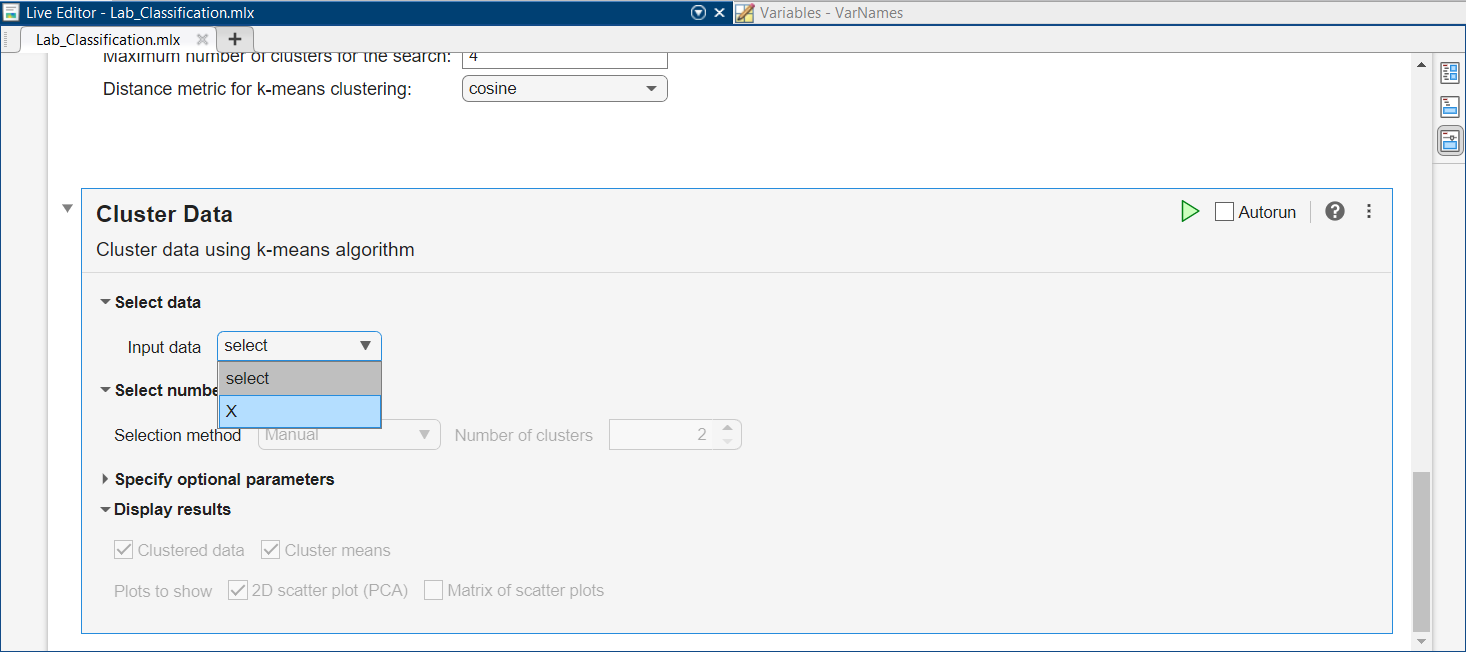
For the Input data, select “X”, containing all $4$ features and $3$ species from Fisher’s Iris data. This will allow you to pick a Selection method for number of clusters using the drop-down list. Pick the “Optimal” method. Leave the default Range from $2$ to $6$.

Recall that when we used the Classification Learner, we also loaded the variable y in the app.

Why are we not loading y in the Cluster Data task?

Among the evaluation criteria, you can spot the Sillhouette method used before, but also $3$ other criteria:

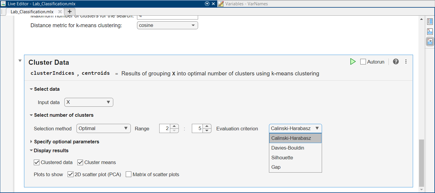
Select the first criterion, then run the task by clicking on the green triangle

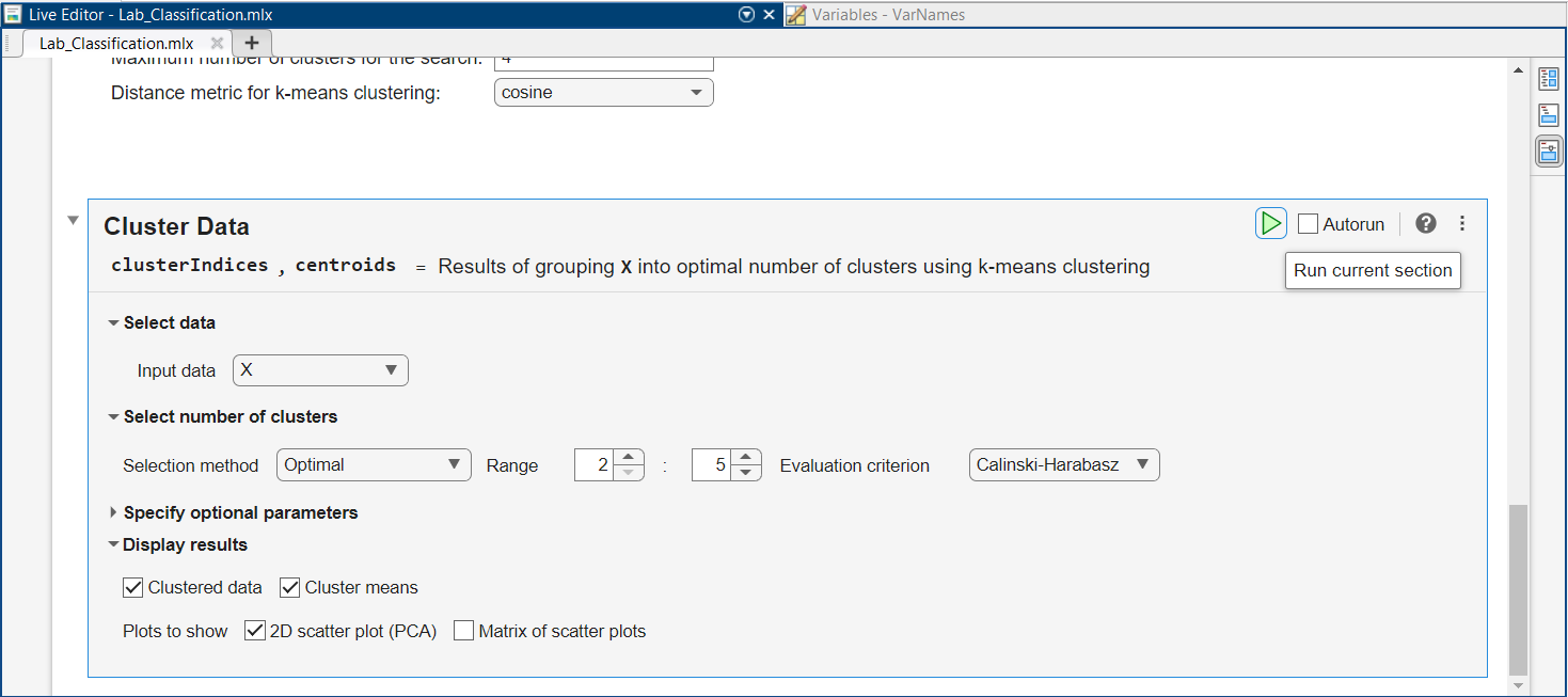
After running the task, scroll down to see the results.

What is the optimal number of clusters selected?

Principal Component Analysis

An important unsupervised learning method is the Principal Component Analysis (PCA). PCA decreases the dimensionality of the data, allowing to vizualize the data easier, and also remove the less important features.

In the case of the Iris dataset, you noticed that in the Cluster Data task, we left the “2D scatter plot (PCA)” as ticked. Scroll to the bottom of the results and inspect the plot of the first 2 PCA components.

What do you think is the difference between visualising the first two principle components as in this figure versus loading just two features, as in the case of Data $1$, $2$ and $3$ loaded above?

To analyse PCA in more detail, scroll below the Cluster Data task, and locate the Reduce Dimensionality task. If we want to reduce dimensionality, we will lose some information. But what if we can maintain almost all information in the data and reduce significantly the dimensions?

Leave the default value of $95\%$ for the Reduction criterion. As before, select “X” as the input and run the task by pressing on the green “play” button.

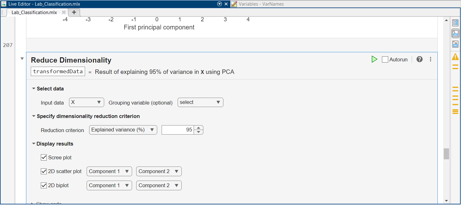
How many components are necessary to explain $95\%$ of the data?

If we reduce the data to this many components, how much memory do we save?

Note that the dimensionality reduction produced a new dataset called “transformedData” (look right under “Reduce Dimensionality”). This is the reduced dataset. Open the Classification Learner again and open a new session which loads “transformedData”. Run some of the previous models on the updated data.

What change do you notice in the performance?

Do you consider that the change in accuracy is justified as tradeoff for the reduced space?

Further more, at the bottom of the script, you can see the PCA biplot. This shows how the four features are positioned in two dimensions relative to the principal components. The for variables Var1-Var4 represent the features. The angles between them show how correlated they are. For example, the biplot tells us that the petal length and petal width, which are the last two features, are highly correlated.

Further Work

You can test the ML models above with different datasets. There are a lot of datasets available online. An example is the default ML datasets on the Mathworks website: https://uk.mathworks.com/help/stats/sample-data-sets.html

To evaluate a new dataset, you can type in the Command Window (locate it using the first figure in this lab script) the commands to load the dataset into the memory. For example, for the ionosphere.mat dataset, type the following in the Command Window and then press Enter:

1
2
clear all; 
load ionosphere.mat;

If the dataset is in the section “Data Sets Available with Specific Examples” from the link above, such as the arrythmia.mat dataset, the data can be loaded by typing the following in the Command Window and then pressing Enter:

1
2
3
clear all; 
openExample("arrhythmia.mat"); 
load arrhythmia.mat;

Notice which new variables are loaded in the Workspace. Now you can repeat the previous experiments with a new dataset. For instance, for the arrhythmia dataset, which has $279$ features, we can run the Reduce Dimensionality task.

Can you find what those features are by inspecting the workspace?

Without loading any other datasets, select the Input data as “X” again and run the task. You may consider unticking the “2D biplot” box, as this can generate errors for some datasets. What is the reduced number of features explaining $95\%$ of the data?

After this, you can also start a new session with the Classification Learner, and load the corresponding new variables in the app to train models as above. Of course, you need to first understand the dataset, and make sure it is compatible with the problem you are trying to solve (classification). For this, you can look at the variables in the Workspace (see the first figure in this lab script), and double click on each one to see their contents. Many of the datasets contain a variable called “Description”, which provides further information.

A full documentation of the Statistics and Machine Learning Matlab Toolbox can be found at: https://uk.mathworks.com/help/stats/index.html. This includes the documentation of all machine learning models supported by the toolbox (including the ones discussed in this lab) and also all functionalities of the Classification Learner Learner app, located in the Classification section of the documentation website.