Electromagnetic Interference: Cable/Data Bus Example

Introduction

The purpose of this laboratory exercise is to look at electromagnetic interference (EMI) effects on a simple multi-conductor connection that might be found in a multiway cable connection or a data bus. EMI is a major cause of performance degradation and measurement error in electronic systems. Indeed EMI issues must be brought down to acceptable levels if a product is to satisfy electromagnetic compatibility (EMC) requirements as part of qualification to be Conformité Européenne (CE) marked and sold legally. The experiments includes detecting and analysing EMI issues. These experiments will build on knowledge gained from Unit EE12002: Fundamentals of engineering and analysis on Circuit Theory on the frequency dependence of capacitance, and on the electromagnetic effects caused by time varying currents flowing in conductors.

EMI is associated with time varying electrical currents whether in the form of pulses (data streams), ac currents or complex analogue signals. A time varying current involves accelerating and decelerating the charge carriers, typically electrons, in a conductor or semiconductor. The resulting gain and loss in the energy of the charge carriers causes the emission of electromagnetic radiation, an effect exploited in antennas and transformers and quantified by Faraday’s Law and Ampère’s Law. This radiation can then be absorbed by wires and circuits in nearby electrical equipment inducing parasitic currents and voltages that corrupt intended signals in that equipment. This can degrade, or even stop, the equipment from functioning properly. As such, EMI is regarded by governments around the world as such a serious problem that many have introduced laws that set stringent limits on the levels of electromagnetic radiation that can be emitted from electronic and electrical equipment. Equipment designs that do not comply with these laws can lead to engineers being fined, and potentially imprisoned.

Objectives

To measure the frequency response of an eight track connection/data bus circuit.
Assess the leakage of signals between the tracks.
Assess the influence of interference from the mains in the experiment and identify the care needed to take meaningful measurement in the Keysight, or any other, Laboratories.

Preparation

Read this script to find out what is needed to do in the Laboratory session.
Develop a simple spreadsheet in which to record measurements to be taken in the Detailed investigation section.
Find out how to produce a plot with logarithmic scales rather than linear scales.

Theory

(a) shows schematically two unconnected coplanar copper conductors on a piece of printed circuit board (PCB). Despite the difference in geometry, the metal-insulator-metal nature of the structure has electrical properties similar to those of a parallel plate capacitor. For example, when one conductor is held at ground potential (i.e. 0 V) and a voltage $V$ is applied to the other there will be an electric field between the conductors as illustrated in (b). On a path between the conductors of length $L$ the electric field is $E~\approx~ V/L$. The electric field is most intense on the shortest direct path between the conductors, and decreases as the path length increases on the longer curved paths.

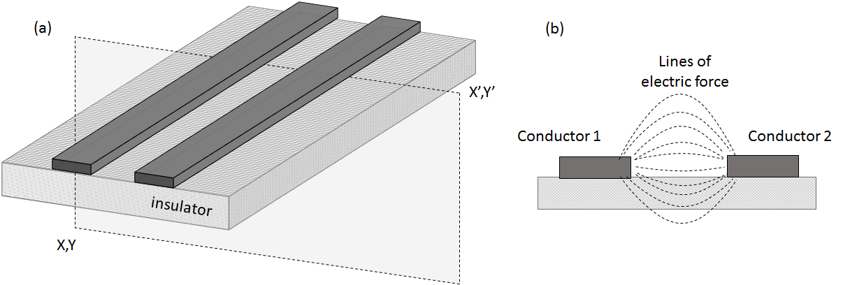
Two parallel straight conductor tracks are shown supported by a flat board. Between the circuit tracks electric field lines are shown which are straight directly between the boards and curve along paths above and below the conductors. The curved paths are naturally longer than the direct path. — Two parallel conductor tracks and the electric field lines likely to be created when a voltage is applied between the tracks.

Two separated conductors, as found in a parallel plate capacitor, will have a capacitance between them. Energy is needed to create an electric field, and the energy stored in a medium with permittivity $\epsilon$ is $U_E \,=\, 1/2 \, \epsilon\, |E|^2$. The energy stored on a capacitance $C$ when a voltage $V$ is applied is $U_c \,=\, 1/2 \, C\, |V|^2$. Equating these energies gives an expression for the capacitance. To do this calculation the rather complicated electric field variation around the conductors needs to be worked out. This is complicated and there is no simple formula for the capacitance. The calculation can require advanced numerical methods and powerful computers. In between parallel tracks on Veroboard measurements and advanced electromagnetic simulations suggest the capacitance per unit length is about 42 pF/m.

The impedance of a capacitor, $C$, at a frequency $f$ is $Z_C ~=~ \frac{1}{j\,2\,\pi\, f \,C}$ and the magnitude or size of the impedance is $|Z_C| ~=~ \frac{1}{2\,\pi \,f \,C}$ The impedance of the capacitor is infinite (open circuit) at zero frequency. The impedance drops with increasing frequency.

Device Under Test (DUT)

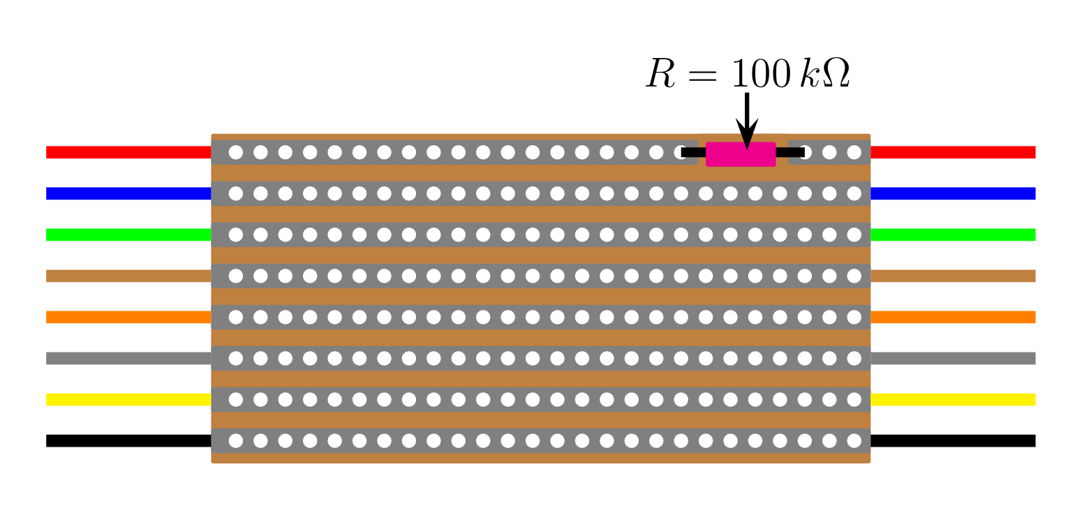
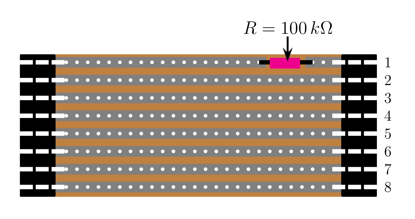
A typical way of making multiple connections between devices is to use multiple parallel tracks, a ribbon cable, or a data bus. In this experiment eight parallel tracks on Veroboard are considered as a multiway connection with one track having a $100\,k\Omega$ resistor soldered into it. There are two types of board. One type has coloured wires attached at the ends as shown in . These boards are about 0.6 m long with an expected capacitance of 25 pF between adjacent tracks. The other type has block connectors soldered to the ends of the veroboard as shown in . These boards are about 0.5 m long with an expected capacitance of 21 pF between adjacent tracks.

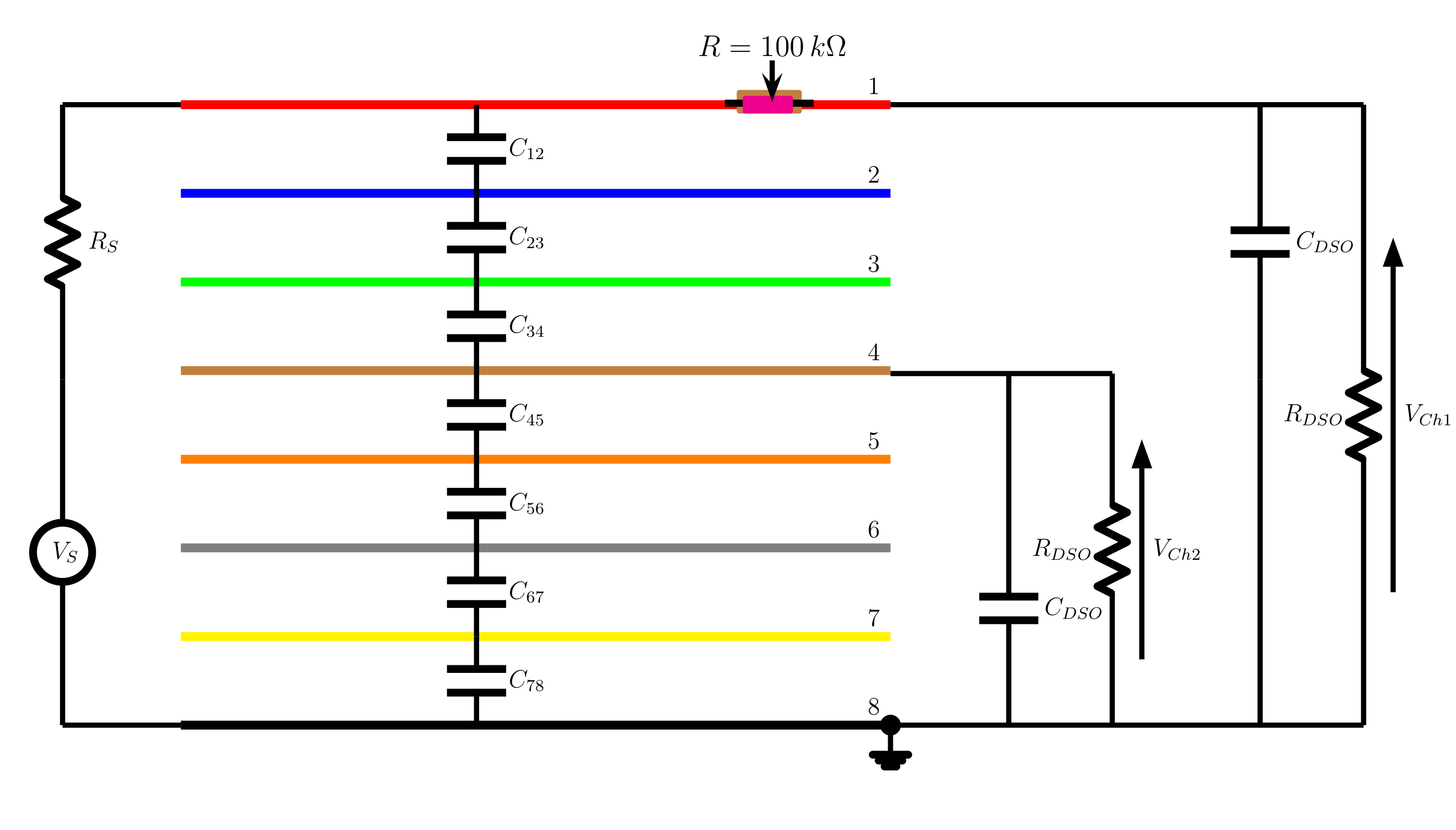
Eight parallel straight conductor tracks are shown on a board. The upper track has a $100\,k\Omega$ resistor soldered across a gap in the track. Each track has wires connected to each end. — Eight-way multi-conductor connection bus on Veroboard with coloured leads.

The electrical schematic of the board is shown in where the source Waveform Generator is connected between one end of circuit track 1 which has the $100\,k\Omega$ resistor, and the end of track number 8. Channel 1 of the Digital Oscilloscope is connected across the other ends of tracks 1 and 8. The Digital Oscilloscope has an input impedance that is comprised of a resistance $R_{DSO} =1\,M\Omega$ in parallel with a capacitance $C_{DSO}=15\,pF$. The connection of the source, the $100\,k\Omega$ resistor and channel 1 of the Digital Oscilloscope forms the primary circuit of this experiment and should be always left connected. Other measurements are taken with Channel 2 of the Digital Oscilloscope connected to conductors 2 to 7, and shows the example where it is connected to track 4.

Circuit diagram showing a voltage source with resistance $R_S$ connected to a $100\,k\Omega$ resistor in track 1 and channel 1 of the oscilloscope connected to the other end of track 1. Adjacent tracks are connected by capacitances. Channel 2 of the oscilloscope is connected to track 4. The oscilloscope connections present a load of their input resistance in parallel with their input capacitance. — Electrical schematic of the eight track Veroboard circuit under test.

Procedure

Initial settings and observation

Connect the circuit board as shown in , but with Channel 2 of the Digital Oscilloscope connected to track 2. The crocodile clip of the oscilloscope probes should be connected to track 8. Placing the eight track veroboard on top of the plastic box that contains all the leads may well make it easier to make the connections required in this experiment.
Set the waveform output on the Waveform Generator : Using the Waveform menu set Sine wave; using the Parameters menu set the output level, $V_g$, to 5 Volts peak to peak, and the signal frequency to 500 Hz; using the Channel menu set the output impedance to $50\,\Omega$ and the Output to ON.
Make sure that both channels 1 and 2 are active on the Digital Oscilloscope so that two waveforms are visible. Selecting Autoscale on the Digital Oscilloscope should show both traces.
Progressively increase the frequency on the Waveform Generator up to 20 MHz while observing the waveform on the Digital Oscilloscope - the timebase will need to be adjusted occasionally so the the waveforms are clear. Note where there are significant changes in the waveform amplitudes and choose a suitable set of frequencies to initially record at.
To make recording data rather easier the Measure facility on the Digital Oscilloscope should be used. Add measures under the Measure menu for the AC-RMS values of both channels 1 and 2. Using the Aquire menu set Aquire Mode to Averaging and using the adjuster knob set the averaging factor to 32.

To measure the frequency response a table of values such as shown below is a clear way of recording the data for the seven connections that are made. Indeed if such a table is set up in a spreadsheet the subsequent graphing of the data is quite easy.

Frequency	$V_1$	$\Delta V_1$	$V_2$	$\Delta V_2$	$V_3$	$\Delta V_3$	$\cdots$	$\cdots$	$V_7$	$\Delta V_7$
(Hz)	(Volts)	(Volts)	(Volts)	(Volts)	(Volts)	(Volts)	$\cdots$	$\cdots$	(Volts)	(Volts)
100	$\vdots$	$\vdots$	$\vdots$	$\vdots$	$\vdots$	$\vdots$	$\cdots$	$\cdots$	$\vdots$	$\vdots$
300	$\vdots$	$\vdots$	$\vdots$	$\vdots$	$\vdots$	$\vdots$	$\cdots$	$\cdots$	$\vdots$	$\vdots$
3000	$\vdots$	$\vdots$	$\vdots$	$\vdots$	$\vdots$	$\vdots$	$\cdots$	$\cdots$	$\vdots$	$\vdots$
$\vdots$	$\vdots$	$\vdots$	$\vdots$	$\vdots$	$\vdots$	$\vdots$	$\cdots$	$\cdots$	$\vdots$	$\vdots$
$\vdots$	$\vdots$	$\vdots$	$\vdots$	$\vdots$	$\vdots$	$\vdots$	$\cdots$	$\cdots$	$\vdots$	$\vdots$
10.0e+06	$\vdots$	$\vdots$	$\vdots$	$\vdots$	$\vdots$	$\vdots$	$\cdots$	$\cdots$	$\vdots$	$\vdots$
20.0e+06	$\vdots$	$\vdots$	$\vdots$	$\vdots$	$\vdots$	$\vdots$	$\cdots$	$\cdots$	$\vdots$	$\vdots$

Measure the frequency response seen at the load end on tracks 1 and 2, noting the accuracy of your measurements.
Measure the frequency responses and their accuracies seen at the load end while track 1 remains connected to channel 1 of the Digital Oscilloscope and channel 2 is connected to tracks 3 to 7.
Plot the data on a single graph for all the responses on tracks 1 to 7 with a logarithmic frequency scale.
Determine if more frequency points are needed, and if needed measure at these frequencies and add these to the plots.
Plot the voltage levels recorded for the outputs of tracks 2 to 7 at a frequency around 1 MHz. Comment on the relationship between the outputs and the significance of the observed leakage of signal between the tracks.

Interference

A common source of interference is the AC mains.

Taking an oscilloscope lead make contact with the probe tip with just a finger and/or thumb. Then press Autoscale on the Digital Oscilloscope and once the Digital Oscilloscope settles look at the amplitude and period of the signal shown and then determine the frequency of this signal.
Under the benches there is a metal bar that supports the bench top. While still maintaining finger/thumb contact with the oscilloscope probe tip, with your other hand take a firm grip of the metal bar that supports the bench top and observe any change in the signal seen on the Digital Oscilloscope .
Note how the interference from the 50 Hz mains in the Laboratory may influence your measures.

Data and observations submission for the Experiment

In addition to making a record of your procedure and results for this experiment in your logbooks please make sure your logbook records include:

Data table recorded in Initial Settings and Observations.
Plot of the frequency response data table recorded in Initial Settings and Observations including accuracy estimations.
Plot of the 1 MHz comparison recorded in Initial Settings and Observations including accuracy estimations.
Comments or observations made on the data recorded in Initial Settings and Observations.
Observations made in Interference.