Frequency Response Measurement

---

Introduction

Almost all circuits have performance that varies with frequency. The frequency response of a circuit or system is commonly used to characterise the performance of the circuit or system. When taking such measurements the accuracy of the measurements needs to be assessed in order to work out how accurate the results are and what can be reliably interpreted from the results. Only if the accuracy is good enough can pass/fail criteria be applied to the performance of the circuit or system.

In this experiment the frequency response of capacitors are investigated as capacitors have a clear and simple frequency response. Measurements are taken of the amplitudes (sizes) of the signals on a Capacitor circuit, and from this current flow and impedance are determined. The accuracy of the Digital Storage Oscilloscope measurement scheme is also assessed.

Not all types of capacitor are identical, and in this experiment measurements are taken with a $1 \,\mu F$ Ceramic capacitor and a $1 \,\mu F$ Tantalum capacitor. It is then possible to see where their performance is the same and where it differs.

Objectives

1. To measure the frequency response of a test Ceramic capacitor circuit.
2. To measure the frequency response of a test Tantalum capacitor circuit.
3. Assess the accuracy of the measurements and identify how stringent a pass/fail test could be undertaken with the measurement setup used in the Keysight Laboratories.

Preparation

1. Read this script to find out what is needed to do in the Laboratory session.
2. Develop a simple spreadsheet in which to record measurements to be taken in the Detailed investigation section.
3. Find out how to produce a plot with logarithmic scales rather than linear scales.
4. Predict the magnitude of the impedance of a $1 \,\mu F$ capacitor at frequencies of $5 kHz$, $100 kHz$ and $5 MHz$ for direct comparison with measurements.

Background

In general a circuit or device will have properties that vary with frequency. In this experiment the properties of the circuit are observed by looking at voltage waveforms at various points in a circuit. The waveforms used in this experiment are sinusoidal single frequency signals which can be written as

\[V(f,t) = V_o\,\cos(2 \, \pi \, f\, t )\]

where $f$ is the frequency, $\omega = 2\, \pi\,f$ is the circular frequency and $t$ is time. The amplitude of this signal is $V_o$. The peak-to-peak voltage of the signal is $2\,V_o$ and the root-mean-square (RMS) voltage is $V_o/\sqrt{2\,}$. RMS voltages are often used and naturally need some averaging to determine their value. As such they can be a more reliable measure than a peak-to-peak which is very susceptible to interference near the peak values in the waveform.

Accuracy in Measurements

All measurement systems suffer from some disturbances that produce inaccuracies or uncertainties in measurements. Noise and interference are common causes of these in electrical and electronic systems. For example when a voltage is read from an instrument that shows just three digits if the instrument reads $1.27$ V the voltage is somewhere in the range $1.265 V$ to $1.27499 V$. There is an inaccuracy of $0.005 V$ and the result can be written as $(1.27 \pm 0.005)$ V. If the instrument is producing values that vary in time somewhat the indicated values might jump around showing $1.25 V$, $1.28 V$, $1.27 V$, $1.26 V$, $1.29 V$. In that case the measured voltage is $(1.27 \pm 0.02)$ V.

Uncertainty in measurements caused by noise are assumed to be random events with a gaussian probability of occurring. This produces indicated measurements with a mean $V_m$ and a standard deviation $\sigma$ and the measurement is then written $V_m \pm \sigma$. Applying gaussian statistics rules, about two thirds of the measures fall within this range, one sixth above the range and one sixth below this range. On a digital readout it is fairly easy to see which decimal place is varying, and ignore any low probability large variations.

Device Under Test (DUT)

The circuit or device that is tested is often referred to as the Device Under Test (DUT). In this experiment the DUT is capacitor. In order to measure current flow a sensing resistor, $R_{sen}$, is connected in series, as shown in .

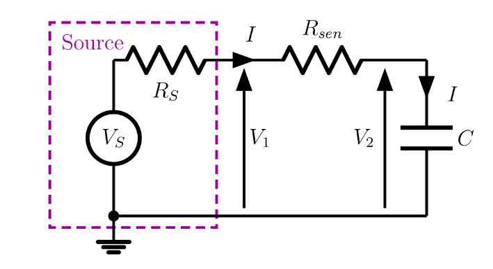
The voltage applied across the capacitor is $V_2$ while the current flow through the capacitor and resistor is \(I = \frac{V_1\,-\,V_2}{R_{sen}}\).

The magnitude of the impedance of the capacitor is easily determined as \(|Z| ~=~ \frac{|V_2|}{|I|}\). Magnitude is used as the current and voltage of the capacitor are in phase quadrature.

The magnitude, or size, of the impedance of the capacitor varies with the frequency, $f$, of the applied signal as

\[|Z_C| ~=~ \frac{|V_2|}{|I|} ~=~ \frac{1}{\omega\,C} ~=~ \frac{1}{2\, \pi\, f \, C }\]

This drops with frequency in an easily identifiable manner.

Procedure

Initial settings and Observations

1. Connect the Output from the Signal Generator to the red and black terminals BreadBoard. The black terminal is the voltage reference for the circuit or Ground. Then using short wires connect the $1 \,\mu F$ Ceramic capacitor and the $100\,\Omega$ sensing resistor to make the circuit shown in .
2. Set the waveform output on the Signal Generator using the Waveform menu. Set Sine wave as the waveform. Using the Parameters menu set the output level to 1.5 Volts peak to peak, and the signal frequency to 500 Hz. Using the Channel menu set the Output to ON.

3. Connect the two channels of the Oscilloscope to the sensing resistor using the oscilloscope leads. Their crocodile clips are ground connections and should be connected to the Ground or voltage reference connection on the circuit. Channel 1 should measure $V_1$ and Channel 2 should measure $V_2$. The oscilloscope probes should be set to $\times 10$ for this experiment, and the Oscilloscope should also be set to use $\times 10$ probe settings. This is set in the Channel menus. These are active when the Channel 1 or Channel 2 buttons are pressed via the Probe menu item and the Entry knob.

   Make sure that both channels 1 and 2 are active on the Oscilloscope so that the $V_1$ and $V_2$ waveforms are visible when the Signal Generator output is switched on.

4. To observe the sinusoidal signals on the Oscilloscope adjust the volts per division to about $1\, V/div$, the timebase to about $1\, msec/div$. Then set the Trigger source to Channel 1 and adjust the Trigger level so that the trigger mark (T) is near the centre of the Channel 1 response. Alternatively select Autoscale on the Oscilloscope to achieve a similar output.
5. To make recording data rather easier the Measure facility on the Oscilloscope should be used. Add measures under the Measure menu for the AC-RMS values of both channels 1 and 2. Using the Aquire menu set Aquire Mode to Averaging and using the Entry knob set the averaging factor to 4.
6. Consider the uncertainty there is in the recordings that can be taken. Measure $V_1$ and the uncertainty, or variability, in $V_1$ with the Signal Generator output set to $1.5\,Vpp$ when the Oscilloscope is set to $10\, V/div$, $1\, V/div$, $0.1\, V/div$ and the maximum sensitivity that can be used while the sinusoidal signal is still within the screen graticule.

Which of these measurement set ups produces the least uncertainty in the measured voltage? Does increasing the Averaging to set the averaging factor to 32 produce more or less uncertainty in the measurement?

Considering how the oscilloscope can be used to measure voltages how is best accuracy achieved?

Detailed investigation

To measure the frequency response a table of values such as shown below is a clear and simple way of recording the data. Indeed if such a table is set up in a spreadsheet the graphing of the data can be done during the experiment and it is then easy to identify where more data points are needed. In addition to the voltages columns should be set up for the DUT current, $I$, and impedance, $Z$:

\[I ~=~ \frac{V_1 \,-\, V_2}{R_{sen}} \qquad \qquad Z ~=~ \frac{V_2}{I}\]

In all cases a column should be included for the uncertainty in the measures. In taking a frequency response it is common to measure at frequencies that are logarithmically spaced. Initially this could be at frequencies that are spaced every decade, or factor of 10, i.e at say $100\, Hz, ~1\,kHz, ~10\,kHz……$ This can be a little coarse so here taking half decade spacing at $100\,Hz, ~300\,Hz, ~1\,kHz, ~3\,kHz……. 10\,MHz, ~20\,MHz$ is advised. $20\,MHz$ is used rather than $30\,MHz$ as $20\,MHz$ the highest frequency the Signal Generator can generate.

Frequency	$V_1$	$\Delta V_1$	$V_2$	$\Delta V_2$	$I = \frac{V_2-V_1}{R_{\text{sen}}}$	$\Delta I$	$Z = \frac{V_2}{I}$	$\Delta Z$
(Hz)	(V)	(V)	(V)	(V)	(A)	(A)	($\Omega$)	($\Omega$)
100
300
1000
$\vdots$	$\vdots$	$\vdots$	$\vdots$	$\vdots$	$\vdots$	$\vdots$	$\vdots$	$\vdots$
$\vdots$	$\vdots$	$\vdots$	$\vdots$	$\vdots$	$\vdots$	$\vdots$	$\vdots$	$\vdots$
3.0e+6
10.0e+6
20.0e+6

If the data in the table is plotted as the experiment is performed it is easy to identify if extra data is needed at intermediate frequencies or if any data points appear to be incorrect. Additional rows are easily inserted into a spreadsheet on a PC/laptop.

Note that a spreadsheet on a PC/laptop does not understand units in items such as $2\,kHz, ~3\,MHz$ or $5\, mV$, these need to be input as $2.0e+3, ~3.0e+6$, or $5.0e-3$.

1. At each frequency measure the RMS (root mean square) of the signals $V_1$, and $V_2$, the uncertainties in the voltages, $\Delta V_1$, and $\Delta V_2$.
2. Plot the data showing $V_1$ and $V_2$ as a function of frequency. Include indication of the accuracy achieved for each of the data points. The frequency ($x$) axis and the voltages ($y$) should be plotted on logarithmic scales to fully observe the data trends.
3. Determine if more frequency points are needed to observe trends in the data, and if needed measure at these frequencies and add these to the plots.
4. Change the DUT capacitor from the $1 \,\mu F$ Ceramic to a $1 \,\mu F$ Tantalum and repeat the measurements and plots.

Further use of the data - is it accurate enough?

To measure the impedances of the capacitors determine the current and impedance

\[I ~=~ \frac{V_1 \,-\, V_2}{R_{sen}} \qquad \qquad Z ~=~ \frac{V_2}{I}\]

and determine the uncertainties in these quantities $\Delta I$ and $\Delta Z$. These evaluations involve taking the differences and ratios of values that have uncertainties, and the basic formulas for evaluating uncertainties in these cases are included in the Appendix.

Plot the current and impedance as a function of frequency including the influence of the uncertainties. Creating columns of $I_m = I \,-\, \Delta I$, $I_p = I \,+\, \Delta I$, $Z_m = Z \,-\, \Delta Z$ and $Z_p = Z \,+\, \Delta Z$ gives a simple illustration of the relative importance of the uncertainties when plotted.

Plotting the impedances of the two different capacitors on the same graph is also informative. An ideal capacitor has an impedance $|Z_C|= 1/(\omega C)$ which drops with frequency. A real capacitor will have a small series inductance from the leads and package. The magnitude of the impedance of an inductor of inductance $L_C$ is $|Z_L| = \omega L_C$ which rises linearly with frequency. The capacitor and series inductor will resonate at a frequency \(f ~=~ \frac{1}{\, 2\, \pi \, \sqrt{L_C\, C\,} \,}\) where the impedance is a minimum. At this frequency impedance of the real capacitor is just a resistance, called the Equivalent Series Resistance (ESR). Determine the inductance $L_C$ of the capacitors and their ESRs.

Data and observations submission for the Experiment

In addition to making a record of your procedure and results for this experiment in your logbooks please make sure your logbook records include:

1. Observations made concerning accuracy in item 6 in Initial Settings and Observations.
2. Data table recorded in Detailed Investigation for both capacitors.
3. Plots of the data recorded in Detailed Investigation with their associated errors and comments or observations made on this data.
4. Plots of the currents and impedances determined from the experimental voltages recorded in Further Use of Data with their observed uncertainty ranges, and comments or observations made on this data.

Appendix - Cumulative Uncertainties

When adding or subtracting values $a \pm \Delta a$ and $b \pm \Delta b$ to determine a result $R = a + b$ or $R = a - b$ the uncertainty, or error, in the result is

\[\Delta R = \sqrt{ \Delta a^2 ~+~ \Delta b^2 \,}\]

When multiplying or dividing values $a \pm \Delta a$ and $b \pm \Delta b$ to determine a result $R = a \times b$ or $R = a/b$ the fractional uncertainty, or error, in the result is

\[\frac{\Delta R}{R} = \sqrt{ \left(\frac{\Delta a}{a}\right)^2 ~+~ \left( \frac{\Delta b}{b} \right)^2 \,}\]

while the uncertainty, or error, in the result is

\[\Delta R ~=~ R ~ \sqrt{ \left(\frac{\Delta a}{a}\right)^2 ~+~ \left( \frac{\Delta b}{b} \right)^2 \,}\]