Branching Brownian motion
Skip to:
Non-mathematical description
Basic mathematical description
My research
Going further
Return to main research page
Non-mathematical description
These descriptions are usually not entirely accurate, and sometimes not at all accurate. They're just stories, not mathematical descriptions.
You've just hosted a party. You wake up the morning after and the house is a tip. You clear the kitchen table to make space for breakfast. Underneath the piles of empty bottles, pringles cans and half-eaten packets of crisps is a thick layer of grime. You put some disinfectant on a cloth and wipe the table, but you miss a patch - in fact you miss a stretch from the middle of the table to the edge. A single bacterium is sitting in the middle of the table, doing what bacteria do - moving around at random, and occasionally splitting into two bacteria, which then move around randomly and occasionally split into two.
Any bacteria that stray away from the unwiped bit of the table and hit the disinfectant die. Do the bacteria eventually die out, or do some of them make it off the table and colonise your kitchen? If they make it to the edge of the table, how long do they take, and how many of them make it?
Every day millions of your cells make copies of their DNA. Millions of cells copying millions of DNA molecules each is pretty complicated, and sometimes little mistakes happen. Usually these make no difference - that's probably one of the reasons why your DNA is such a long string of molecules, so that if there are a few mistakes it doesn't really matter. But over time these little mistakes can slowly make a big difference to your DNA.
Think of the squirrel. Back in the day, squirrels were reddish-brown, to blend in with the trees and leaves in autumn. Then industrialisation happened, and stuff like trees turned grey. All these little mistakes in squirrel DNA had been happening for thousands of years, but now any little mistake that made a squirrel slightly greyer meant that that squirrel had more chance of surviving and breeding. And gradually, in this way, the change in the environment meant that certain little mistakes lived on in the population, and squirrels became grey.
How quickly can this happen? If the environment changes too much too fast, then animals die out, so how quickly can we afford to change the world without causing mass extinctions? On the other hand sometimes we want to make animals, or plants, or fungi, or bacteria, that behave a certain way: then how fast should we change their environment so that they will adapt as quickly as possible without all dying out? Or if we've got something that we want die out before it has a chance to adapt - like bacteria or cancer cells - then by how much do we have to change its environment? Bearing in mind that its environment could be someone's body, we probably want to change the environment as little as possible while still making sure that the organism dies out.
One mathematical way of looking at these questions is to consider branching Brownian motions or branching random walks. These models involve particles (like bacteria) moving around randomly and occasionally splitting into two (or more) new particles. (This immediately looks like a pretty good model for the bacteria-on-a-table picture above; maybe it's not so clear for the DNA picture. But DNA is just a long string of molecules, and we can think of a long string of molecules as a long string of numbers, and think of that long string of numbers as a position in space, so little mistakes in the DNA mean little movements.)
Basic mathematical description
These descriptions may contain some small inaccuracies in order to keep the discussion at a basic level.
To know what a branching Brownian motion is, you need to know what a Brownian motion is. It's a function B:[0,\infty) --> R. It starts from zero, i.e. B(0)=0. It's continuous (you can draw it without taking your pen off the paper). It has independent increments - that means that if t>s, then B(t)-B(s) and B(s)-B(0) are independent, and if t>s>r then B(t)-B(s), B(s)-B(r) and B(r)-B(0) are independent, and so on. And if t>s then B(t)-B(s) is normally distributed (aka Gaussian) with mean 0 and variance t-s.
It's not at all clear that such a thing exists, but it does. If you're wondering what it looks like, it wiggles up and down a lot very fast, usually without going anywhere very quickly.
Now, start a Brownian motion. But then take an independent exponentially distributed random variable with mean 1. Call this random variable T. After time T, we stop our Brownian motion and throw it away. But in its place we put two independent Brownian motions (instead of starting from 0 at time 0, they start from B(T) at time T). And for each of these Brownian motions take an independent exponentially distributed random variable with mean 1. Say one of the new BMs has exponential random variable T'. Then at time T+T', remove that BM and replace it with two new independent ones. And at time T+T'' remove the other BM and replace it with two new independent ones. And keep doing this for each new Brownian motion. You very quickly end up with lots of Brownian motions running around.
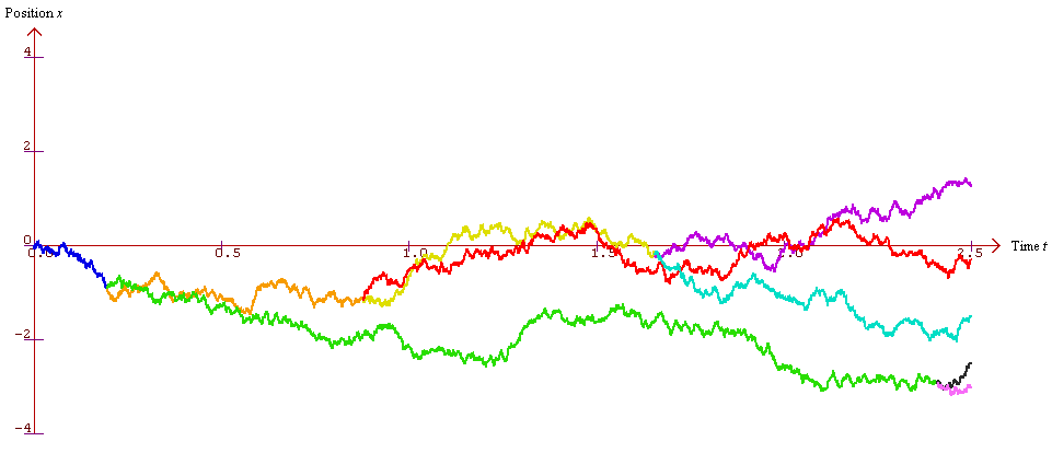
The picture above shows the beginnings of a branching Brownian motion. We start off with the blue Brownian motion; after a while we replace it with the orange and green ones; next the orange one's exponential clock rings, and we replace it with yellow and red; and so on. The picture below shows what things look like if we zoom out.
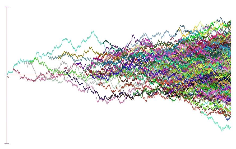
It looks like there's some kind of triangular shape appearing. One way of turning that into maths is to let M(t) be the position of the topmost particle at time t, and ask whether M(t)/t converges to a limit. It's not too hard to show that it does, and the limit is the square root of 2. Then all sorts of questions emerge. Does M(t) really look like sqrt(2)t, or is it more like sqrt(2)t + f(t) for some function f(t) that could still be quite big but which satisfies f(t)/t --> 0 as t --> infinity? Each particle is a Brownian motion, so how on earth did anyone get up near sqrt(2)t? Did they stay near the top of the triangle all the way, or did they hang around in the mass of particles in the middle and then shoot up just before time t? What do the paths of other particles look like - if I give you a function g, are there particles whose paths stay near g?
My research
Again, these descriptions may contain inaccuracies in order to keep the discussion at a basic level. If you want a precise discussion, then you'll have to read the papers!
Let's look at the questions above.
Does M(t) really look like sqrt(2)t, or is it more like sqrt(2)t + f(t) for some function f(t) that could still be quite big but which satisfies f(t)/t --> 0 as t --> infinity?
Maury Bramson showed in 1978 that "M(t) looks like sqrt(2)t - 3log(t)/2sqrt(2) in probability". Then in 2009 Yueyun Hu and Zhan Shi showed that there are actually fluctuations in M(t): although M(t) looks like sqrt(2)t - 3log(t)/2sqrt(2) most of the time, occasionally a particle travels much further, and at these times M(t) looks like sqrt(2)t - log(t)/2sqrt(2). These are two of my favourite results about BBM (actually Hu and Shi proved theirs for the effectively more general model of branching random walk), and if you don't already have favourite results about BBM then I recommend these! On the downside, if you want to read the proofs, each is more than 40 pages long. Luckily I've written short proofs of both, clocking in at 18 pages combined. See my paper A simple path to asymptotics for the frontier of a branching Brownian motion.
Each particle is a Brownian motion, so how on earth did anyone get up near sqrt(2)t? Did they stay near the top of the triangle all the way, or did they hang around in the mass of particles in the middle and then shoot up just before time t?
The answer to "how on earth did a Brownian motion get up near sqrt(2)t" is simply that at time t there are something like e^t Brownian motions hanging around, all somewhat independent, so it's quite likely that some of them have managed to get a long way away from 0. But no particles stay with a constant times log(t) of sqrt(2)t for all t. If you want particles to stay near sqrt(2)t for all t, the best you can do is a constant times t^(1/3). There are several relevant papers here, by Fang and Zeitouni, Faraud, Hu and Shi, Jaffuel, and to a lesser extent Harris and Roberts. And if you want to know what particles near M(t) look like, well, they stay around s^(1/2) below sqrt(2)s for s < t/2, and (t-s)^(1/2) of sqrt(2)s for s > t/2. This is a very rough approximation. The papers of Arguin, Bovier and Kistler - for example The genealogy of extremal particles of Branching Brownian Motion - will give you a better idea.
What do the paths of other particles look like - if I give you a function g, are there particles whose paths stay near g?
Now, here is where Harris and Roberts - The unscaled paths of branching Brownian motion really helps. The answer obviously depends on g, so it's a bit complicated, but for reasonable g we can tell you not only "yes" or "no" but if yes, then how many particles stay near g up to time t, and if no, then what is the probability of there being someone who has stayed near g up to time t. If you prefer the large deviations-style picture, where your function g is on [0,1] and the paths of particles are rescaled, then you can instead look at Branching Brownian motion: Almost sure growth along scaled paths.
Going further
We can get a bit more creative with the model. We don't have to insist that every particle has exactly two offspring: the number of offspring can be random, and might depend on the position of the particle at the fission time. Similarly the rate at which particles split might depend on their position. We can ask what the process looks like from the point of view of the topmost particle - what is the distribution of the second topmost particle for example? There's a lot of work going on in this area now.
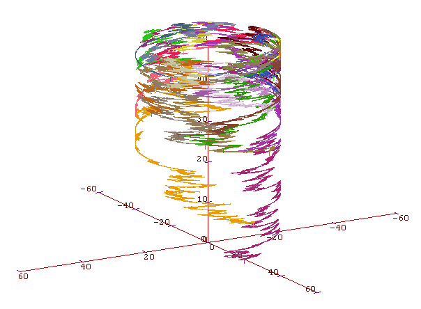
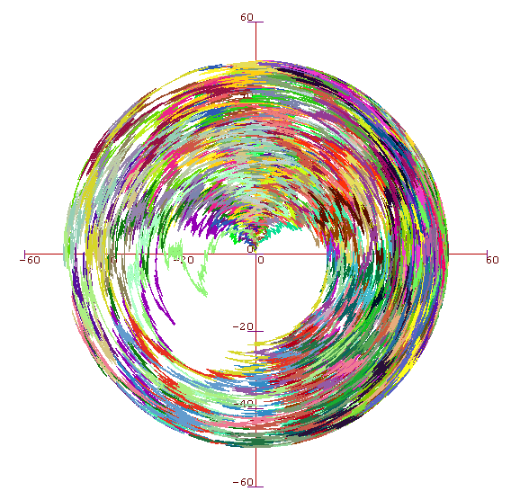
Here's another question that I thought about for a very short while a couple of years ago. Imagine we run a BBM on a circle (ie take positions modulo 2π). Imagine time as the radius of our circle, and draw the path of each particle in black. We end up with a subset of the plane marked in black. There is a unique white component that contains (0,-a) for all small a. What is the area of this component? If we draw the path of each particle as a line (or sausage) of width delta, what is the area of the set of all white points in the plane? What if delta=delta(t) is a decreasing function of t? For example we might take delta(t)=e^(-t).
Here's a picture up to t=50, although for aesthetic purposes I drew each particle in a different colour, rather than drawing them all in black.
It may be easier to think of time as a third spatial dimension, in which case our picture looks like a cylinder.