3 Markov chains
Discrete-time countable-state-space basics:
Markov property, transition matrices;
irreducibility and aperiodicity;
transience and recurrence;
equilibrium equations and convergence to equilibrium.
Discrete-time countable-state-space: why ‘limit of sum need not always equal sum of limit.’
Continuous-time countable-state-space: rates and \(Q\)-matrices.
Definition and basic properties of Poisson counting process.
Instead of “countable-state-space” Markov chains, we’ll use the shorter phrase “discrete Markov chains” or “discrete space Markov chains.”
If some of this material is not well-known to you, then invest some time in looking over (for example) chapter 6 of Grimmett and Stirzaker (2001).
3.1 Basic properties for discrete time and space case
Markov chain \(X=\{X_0, X_1, X_2, \ldots\}\): we say that \(X\) at time \(t\) is in state \(X_t\).
\(X\) must have the Markov property: \[p_{xy}=p(x,y)=\operatorname{\mathbb{P}}\left(X_{t+1}=y \mid X_t=x, X_{t-1}, \ldots\right)\] must depend only on \(x\), \(y\), not on rest of past. (Our chains will be time-homogeneous, meaning no \(t\) dependence either.)
View states \(x\) as integers. More general countable discrete state-spaces can always be indexed by integers.
We will soon see an example, “Markov’s other chain,” showing that we need to insist on the possibility of conditioning by further past \(X_{t-1}, \ldots\) in the definition.
Chain behaviour is specified by (a) initial state \(X_0\) (could be random) and (b) table of transition probabilities \(p_{xy}\).
Important matrix structure: if \(p_{xy}\) are arranged in a matrix \(P\) then \((i,j)^{\text{th}}\) entry of \(P^n=P \times \ldots \times P\) (\(n\) times) is \(p^{(n)}_{ij}=\operatorname{\mathbb{P}}\left(X_{n}=j|X_0=i\right)\).
Equivalent: Chapman-Kolmogorov equations \[ p^{(n+m)}_{ij} = \sum_k p^{(n)}_{ik}p^{(m)}_{kj}. \]
Note \(\sum_y p_{xy}=1\) by “law of total probability.”
Test understanding: show how the Chapman-Kolmogorov equations follow from considerations of conditional probability and the Markov property.
3.2 Example: Models for language following Markov
How to generate “random English” as a Markov chain:
Take a large book in electronic form, for example Tolstoy’s “War and Peace” (English translation).
Use it to build a table of digram frequencies (digram \(=\) pair of consecutive letters).
Convert frequencies into conditional probabilities of one letter following another, and use these to form a Markov chain to generate “random English.”
It is an amusing if substantial exercise to use this as a prior for Bayesian decoding of simple substitution codes.
To find a large book, try Project Gutenberg.
Skill is required in deciding which characters to use: should one use all, or some, punctuation? Certainly need to use spaces.
Trigrams would be more impressive than digrams. Indeed, one needs to work at the level of words to simulate something like English. Here is example output based on a children’s fable:
It was able to the end of great daring but which when Rapunzel was a guardian has enjoined on a time, after a faked morning departure more directly; over its days in a stratagem, which supported her hair into the risk of endless figures on supplanted sorrow. The prince’s directive, to clamber down would come up easily, and perceived a grudge against humans for a convincing simulation of a nearby robotic despot. But then a computer typing in a convincing simulation of the traditional manner. However they settled in quality, and the prince thought for Rapunzel made its ward’s face, that as she then a mere girl.
- Here are some word transition probabilities from the source used for the above example: \[P(\text{round}|\text{all}) = P(\text{contact}|\text{all}) = 0.50\] \[P(\text{hearing}|\text{ocean,}) = P(\text{first,}|\text{go})=1.00\] \[P(\text{As}|\text{up.}) = P(\text{Every}|\text{day.})=1.00 \] \[P(\text{woman}|\text{young}) = P(\text{prince.}|\text{young}) = P(\text{man}|\text{young}) =0.33.\]
3.3 (Counter)example: Markov’s other chain
Conditional probability can be subtle. Consider:
Independent Bernoulli \(X_0, X_2, X_4, \ldots\) such that \(\operatorname{\mathbb{P}}\left(X_{2n}=\pm 1\right)=\tfrac12\);
Define \(X_{2n+1}=X_{2n}X_{2n+2}\) for \(n=0, 1, \ldots\); these also form an independent identically distributed sequence.
\(\operatorname{\mathbb{P}}\left(X_{n+1}=\pm 1|X_n\right)=\tfrac12\) for any \(n\geq1\).
Chapman-Kolmogorov equations hold for any \(0\leq k \leq n+k\): \[ \operatorname{\mathbb{P}}\left(X_{n+k}=\pm 1|X_0\right) = \sum_{y=\pm1} \operatorname{\mathbb{P}}\left(X_{n+k}=\pm 1|X_k=y\right)\operatorname{\mathbb{P}}\left(X_{k}=y|X_0\right)\,. \]
Nevertheless, \(\operatorname{\mathbb{P}}\left(X_2=\pm 1 | X_1=1, X_0=u\right)\) depends on \(u=\pm1\), so Markov property fails for \(X\)
This example is taken from Grimmett and Stirzaker (2001).
Note that, although \(X_0, X_2, X_4, \ldots\) are independent and \(X_1,X_3,X_5,\ldots\) are independent, the entire sequence of random variables \(X_0, X_1, X_2, \ldots\) are most certainly not independent!
Test understanding by checking the calculations above.
It is usual in stochastic modelling to start by specifying that a given random process \(X=\{X_0, X_1, X_2, \ldots\}\) is Markov, so this kind of issue is not often encountered in practice. However it is good to be aware of it: conditioning is a subtle concept and should be treated with respect!
3.4 Irreducibility and aperiodicity
- A discrete Markov chain is irreducible if for all \(i\) and \(j\) it has a positive chance of visiting \(j\) at some positive time, if it is started at \(i\).
Consider the word game: change “good” to “evil” through other English words by altering just one letter at a time. Illustrative question (compare Gardner (1996)): does your vocabulary of 4-letter English words form an irreducible Markov chain under moves which attempt random changes of letters? You can find an algorithmic approach to this question in Knuth (1993).
- It is aperiodic if one cannot divide state-space into non-empty subsets such that the chain progresses through the subsets in a periodic way. Simple symmetric walk (jumps \(\pm1\)) is not aperiodic.
Equivalent definition: an irreducible chain \(X\) is aperiodic if its “independent double” \(\{(X_0, Y_0), (X_1, Y_1), \ldots\}\) (for \(Y\) an independent copy of \(X\)) is irreducible.
- If the chain is not irreducible, then we can compute the chance of it getting from one state to another using first passage equations: if \[ f_{ij} = \operatorname{\mathbb{P}}\left(X_n=j \text{ for some positive } n | X_0=i\right) \] then solve linear equations for the \(f_{ij}\)
Because of the connection with matrices noted above, this can be cast in terms of rather basic linear algebra. First passage equations are still helpful in analyzing irreducible chains: for example the chance of visiting \(j\) before \(k\) is the same as computing \(f_{ij}\) for the modified chain which stops on hitting \(k\).
3.5 Example: Markov tennis
How does probability of win by \(B\) depend on \(p=\operatorname{\mathbb{P}}\left(B \text{ wins point}\right)\)?
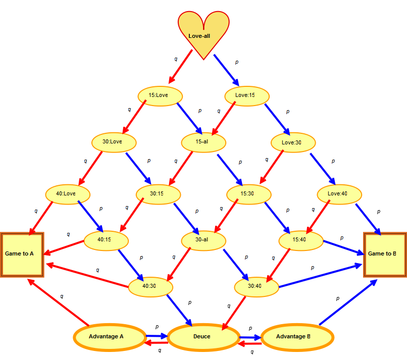
Use first passage equations, then solve linear equations for the \(f_{ij}\), noting in particular \[f_{\text{ Game to A},\text{Game to B}}=0\,, \qquad f_{\text{ Game to B},\text{Game to B}}=1\,.\]
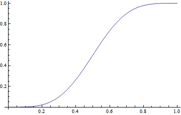
I obtain \[ f_{\text{ Love-All},\text{Game to B}}\quad=\quad\tfrac{p^4 (15 - 34 p + 28 p^2 - 8 p^3)}{1 - 2 p + 2 p^2}\,, \] graphed against \(p\) below:
3.6 Transience and recurrence
Is it possible for a Markov chain \(X\) never to return to a starting state \(i\,\)? If so then that state is said to be transient.
Otherwise the state is said to be recurrent.
Moreover if the return time \(T\) has finite mean then the state is said to be positive-recurrent.
Recurrent states which are not positive-recurrent are called null-recurrent.
States of an irreducible Markov chain are all recurrent if one is, all positive-recurrent if one is.
Because of this last fact, we often talk about recurrent chains and transient chains rather than recurrent states and transient states.
Asymmetric simple random walk (jumps \(\pm1\) with prob \(\neq 1/2\) of \(+1\)) is an example of a transient Markov chain: see Cox and Miller (1965) for a pretty explanation using strong law of large numbers.
Symmetric simple random walk (jumps \(\pm1\) with prob \(1/2\) each) is an example of a (null-)recurrent Markov chain.
We will see later that there exist infinite positive-recurrent chains.
Terminology is motivated by the limiting behaviour of probability of being found in that state at large time. Asymptotically zero if null-recurrent or transient; tends to \(1/\operatorname{\mathbb{E}}\left[T\right]\) if aperiodic positive-recurrent.
The fact that either all states are recurrent or all states are transient is based on the criterion for recurrence of state \(i\), \[\sum_n p^{(n)}_{ii}=\infty,\] which in turn arises from an application of generating functions. The criterion amounts to asserting, the chain is sure to return to a state \(i\) exactly when the mean number of returns is infinite.
3.7 Recurrence/transience for random walks on \(\mathbb Z\)
Let \(X\) be a random walk on \(\mathbb Z\) which takes steps of size 1 with probability \(p\) and minus one with probability \(q=1-p\). Define \(T_{0,1}\) to be the first time at which \(X\) hits 1, if it starts at 0.
Note that it’s certainly possible to have \(\operatorname{\mathbb{P}}\left(T_{0,1}<\infty\right)<1\), that is, for the random variable \(T_{0,1}\) to take the value \(\infty\)!
The probability generating function for this random variable satisfies \[ G(z) = \operatorname{\mathbb{E}}\left[z^{T_{0,1}}\right] =zp+zq G(z)^2 \] Solving this (and noting that we need to take the negative root!) we see that \[ G(z) = \frac{1-\sqrt{1-4pqz^2}}{2qz} \,, \] and so \(\operatorname{\mathbb{P}}\left(T_{0,1}<\infty\right) = \lim_{z\to 1}G(z) = \min\{p/q,1\}\). Thus if \(p<1/2\) there is a positive chance that \(X\) never reaches state 1; by symmetry, \(X\) is recurrent iff \(p=1/2\).
- Test understanding: Show that the quadratic formula for \(G(z)\) holds by considering what can happen at time 1: argue that if \(X_1=-1\) the time taken to get from \(-1\) to \(1\) has the same distribution as the time taken to get from \(-1\) to 0 plus the time to get from 0 to 1; these random variables are independent, and so the pgf of the sum is easy to work with…
- If we take the positive root then \(G(z)\to\infty\) as \(z\to 0\), rather than to 0!
- Here we are using the fact that, since our state space is irreducible, state \(i\) is recurrent iff \(\operatorname{\mathbb{P}}\left(T_{i,j}<\infty\right)=1\) for all states \(j\), where \(T_{i,j}\) is the first time that \(X\) hits \(j\) when started from \(i\).
3.8 Equilibrium of Markov chains
- If \(X\) is irreducible and positive-recurrent then it has a unique equilibrium distribution \(\pi\): if \(X_0\) is random with distribution given by \(\operatorname{\mathbb{P}}\left(X_0=i\right)=\pi_i\) then \(\operatorname{\mathbb{P}}\left(X_n=i\right)=\pi_i\) for any \(n\).
In general the chain continues moving, it is just that the marginal probabilities at time \(n\) do not change.
- Moreover the equilibrium distribution viewed as a row vector solves the equilibrium equations: \[ \pi P =\pi \,, \qquad\text{ or }\quad \pi_j = \sum_i \pi_i p_{ij}\,. \]
Test understanding: Show that the \(2\)-state Markov chain with transition probability matrix \[\left(\begin{matrix} 0.1 & 0.9\\ 0.8 & 0.2 \end{matrix}\right)\] has equilibrium distribution \[\pi=(0.470588\ldots, 0.529412\ldots).\] Note that you need to use the fact that \(\pi_1+\pi_2=1\): this is always an important extra fact to use in determining a Markov chain’s equilibrium distribution!
- If in addition \(X\) is aperiodic then the equilibrium distribution is also the limiting distribution (for any \(X_0\)): \[\operatorname{\mathbb{P}}\left(X_n=i\right)\to \pi_i \quad\text{ as }n\to\infty\,.\]
This limiting result is of great importance in MCMC. If aperiodicity fails then it is always possible to sub-sample to convert to the aperiodic case on a subset of state-space.
The note at the end of the previous section shows the possibility of computing mean recurrence time using matrix arithmetic.
NB: \(\pi_i\) can also be interpreted as “mean time in state \(i\).”
3.9 Sums of limits and limits of sums
Finite state-space discrete Markov chains have a useful simplifying property: they are always positive-recurrent if they are irreducible.
This can be proved by using a result, that for null-recurrent or transient states \(j\) we find \(p^{(n)}_{ij}\to0\) as \(n\to\infty\), for all other states \(i\). If there were null-recurrent or transient states in a finite state-space discrete Markov chain, this would give a contradiction: \[ \sum_{j}\lim_{n\to\infty}p^{(n)}_{ij} = \lim_{n\to\infty}\sum_{j}p^{(n)}_{ij} \] and the right-hand sum equals \(1\) from “law of total probability,” while left-hand sum equals \(\sum0=0\) by null-recurrence.
This argument doesn’t give a contradiction for infinite state-space chains as it is incorrect arbitrarily to exchange infinite limiting operations: \(\lim\sum \neq \sum\lim\) in general.
Some argue that all Markov chains met in practice are finite, since we work on finite computers with finite floating point arithmetic. Do you find this argument convincing or not?
Recall from the “Limits versus expectations” section the principal theorems which deliver checkable conditions as to when one can swap limits and sums.
3.10 Continuous-time countable state-space Markov chains (a rough guide)
This is a very rough guide, and much of what we will talk about in the course will be in discrete time. However, sometimes the easiest examples in Markov chains are in continuous-time. The important point to grasp is that if we know the transition rates \(q(x,y)\) then we can write down differential equations to define the transition probabilities and so the chain. We don’t necessarily try to solve the equations…
Definition of continuous-time (countable) discrete state-space (time-homogeneous) Markov chain \(X=\{X_t:t\geq0\}\): for \(s, t>0\) \[ p_t(x,y)= \operatorname{\mathbb{P}}\left(X_{s+t}=y|X_s=x, X_{u} \text{ for various }u\leq s\right) \] depends only on \(x\), \(y\), \(t\), not on rest of past.
Organize \(p_t(x,y)\) into matrices \(P(t)=\{p_t(x,y): \text{ states }x,y\}\); as in discrete case \(P(t)\cdot P(s)=P(t+s)\) and \(P(0)\) is identity matrix.
(Try to) compute time derivative: \(Q=(d/dt)P(t)|_{t=0}\) is matrix of transition rates \(q(x,y)\).
For short, we can write \[p_t(x,y)=\operatorname{\mathbb{P}}\left(X_{s+t}=y|X_s=x, \mathcal{F}_s\right)\] where \(\mathcal{F}_s\) represents all possible information about the past at time \(s\).
From here on we omit many “under sufficient regularity” statements. Norris (1998) gives a careful treatment.
The row-sums of \(P(t)\) all equal \(1\) (“law of total probability”). Hence the row sums of \(Q\) ought to be \(0\) with non-positive diagonal entries \(q(x,x)=-q(x)\) measuring rate of leaving \(x\).
For suitably regular continuous-time countable state-space Markov chains, we can use the \(Q\)-matrix \(Q\) to simulate the chain as follows:
rate of leaving state \(x\) is \(q(x)=\sum_{y\neq x}q(x,y)\) (since row sums of \(Q\) should be zero). Time till departure is Exponential\((q(x))\);
on departure from \(x\), go straight to state \(y\neq x\) with probability \(q(x,y)/q(x)\).
Why an exponential distribution? Because an effect of the Markov property is to require the holding time until the first transition to have a memory-less property – which characterizes Exponential distributions.
Here it is relevant to note that “minimum of independent Exponential random variables is Exponential.”
Note that there are two strong limitations of continuous-time Markov chains as stochastic models: the Exponential distribution of holding times may be unrealistic; and the state to which a transition is made does not depend on actual length of holding time (this also follows rather directly from the Markov property). Of course, people have worked on generalizations (keyword: semi-Markov processes).
- Compute the \(s\)-derivative of \(P(s)\cdot P(t)=P(s+t)\). This yields the famous Kolmogorov backwards equations: \[ Q\cdot P(t) = P(t)^{\prime}\,. \] The other way round yields the Kolmogorov forwards equations: \[ P(t)\cdot Q = P(t)^{\prime}\,. \]
Test understanding: use calculus to derive \[\begin{align*} \sum_z p_s(x,z) p_t(z, y) &= p_{s+t}(x,y) \text{ gives } \sum_z q(x,z) p_t(z, y) = \frac{\partial}{\partial t}p_t(x,y) \,,\\ \sum_z p_t(x,z) p_s(z, y) &= p_{t+s}(x,y) \text{ gives } \sum_z p_t(x, z) q(z,y) = \frac{\partial}{\partial t}p_t(x,y)\,. \end{align*}\] Note the shameless exchange of differentiation and summation over potentially infinite state-space…
- If statistical equilibrium holds then the transition probabilities should converge to limiting values as \(t\to\infty\): applying this to the forwards equation we expect the equilibrium distribution \(\pi\) to solve \[\pi\cdot Q = \mathbf{0}\,.\]
Test understanding: applying this idea to the backwards equation gets us nothing, as a consequence of the vanishing of row sums of \(Q\).
In extended form \(\pi\cdot Q=\mathbf{0}\) yields the important equilibrium equations \[\sum_z \pi(z) q(z,y) = 0\,.\]
3.11 Example: the Poisson process
We use the above theory to define chains by specifying the non-zero rates. Consider the case when \(X\) counts the number of people arriving at random at constant rate:
Stipulate that the number \(X_t\) of people in system at time \(t\) forms a Markov chain.
Transition rates: people arrive one-at-a-time at constant rate, so \(q(x,x+1)=\lambda\).
One can solve the Kolmogorov differential equations in this case: \[ \operatorname{\mathbb{P}}\left(X_t=n| X_0=0\right) = \frac{(\lambda t)^n}{n!}e^{-\lambda t}\,. \]
For most Markov chains one makes progress without solving the differential equations.
The interplay between the simulation method above and the distributional information here is exactly the interplay between viewing the Poisson process as a counting process (“Poisson counts”) and a sequence of inter-arrival times (“Exponential gaps”). The classic relationships between Exponential, Poisson, Gamma and Geometric distributions are all embedded in this one process.
Two significant extra facts are
superposition: independent sum of Poisson processes is Poisson;
thinning: if arrivals are censored i.i.d. at random then result is Poisson.
3.12 Example: the M/M/1 queue
Consider a queue in which people arrive and are served (in order) at constant rates by a single server.
Stipulate that the number \(X_t\) of people in system at time \(t\) forms a Markov chain.
Transition rates (I): people arrive one-at-a-time at constant rate, so \(q(x,x+1)=\lambda\).
Transition rates (II): people are served in order at constant rate, so \(q(x,x-1)=\mu\) if \(x>0\).
One can solve the equilibrium equations to deduce: the equilibrium distribution of \(X\) exists and is Geometric if and only if \(\lambda<\mu\).
Don’t try to solve the equilibrium equations at home (unless you enjoy that sort of thing). In this case it is do-able, but during the module we’ll discuss a much quicker way to find the equilibrium distribution in favourable cases.
Here is the equilibrium distribution in more explicit form: in equilibrium \[\operatorname{\mathbb{P}}\left(X=x\right) = (1-\rho)\rho^x \qquad\text{ for } x=0, 1, 2, \ldots\] where \(\rho=\lambda/\mu\in(0,1)\) (the traffic intensity).