2 Expectation and probability
For most APTS students most of this material should be well-known:
Probability and conditional probability;
Basic expectation and conditional expectation;
discrete versus continuous (sums and integrals);
limits versus expectations.
It is set out here, describing key ideas rather than details, in order to establish a sound common basis for the module.
This material uses a two-part format. The main text presents the theory, often using itemized lists. Indented panels such as this one present commentary and useful exercises (announced by “Test understanding”). It is likely that you will have seen most, if not all, of the preliminary material at undergraduate level. However syllabi are not uniform across universities; if some of this material is not well-known to you then:
read through it to pick up the general sense and notation;
supplement by reading (for example) the first five chapters of Grimmett and Stirzaker (2001).
2.1 Probability
Sample space \(\Omega\) of possible outcomes;
Probability \(\mathbb{P}\) assigns a number between \(0\) and \(1\) inclusive (the probability) to each (sensible) subset \(A\subseteq\Omega\) (we say \(A\) is an event);
Advanced (measure-theoretic) probability takes great care to specify what sensible means: \(A\) has to belong to a pre-determined \(\sigma\)-algebra \(\mathcal{F}\), a family of subsets closed under countable unions and complements, often generated by open sets. We shall avoid these technicalities, though it will later be convenient to speak of \(\sigma\)-algebras \(\mathcal{F}_t\) as a shorthand for “information available by time \(t\).”
Rules of probability:
Normalization: \(\mathbb{P}(\Omega)=1\);
\(\sigma\)-additivity: if \(A_1\), \(A_2\) … form a disjoint sequence of events then \[\mathbb{P}( A_1 \cup A_2 \cup \dots)= \sum_i \mathbb{P}(A_i)\,.\]
Example of a sample space: \(\Omega=(-\infty, \infty)\).
To define a probability \(\mathbb{P}\), we could for example start with \[\operatorname{\mathbb{P}}\left((a,b)\right)=\tfrac{1}{\sqrt{2\pi}}\int_a^be^{-u^2/2}\operatorname{d}\hspace{-0.6mm}u\] and then use the rules of probability to determine probabilities for all manner of sensible subsets of \((-\infty, \infty)\).
In this example a “natural” choice for \(\mathcal{F}\) is the family of all sets generated from intervals by indefinitely complicated countably infinite combinations of countable unions and complements.
Test understanding: use the rules of probability to explain
why \(\operatorname{\mathbb{P}}\left(\emptyset\right)=0\),}
why \(\operatorname{\mathbb{P}}\left(A^c\right)=1-\operatorname{\mathbb{P}}\left(A\right)\) if \(A^c=\Omega\setminus A\), and
why it makes no sense in general to try to extend \(\sigma\)-additivity to uncountable unions such as \((-\infty, \infty)=\bigcup_x\{x\}\).
2.2 Conditional probability
- We declare the conditional probability of \(A\) given \(B\) to be \(\mathbb{P}(A|B)=\mathbb{P}(A\cap B)/\mathbb{P}(B)\), and declare the case when \(\mathbb{P}(B)=0\) as undefined.
Actually we often use limiting arguments to make sense of cases when \(\operatorname{\mathbb{P}}\left(B\right)=0\).
Bayes: if \(B_1, B_2, \dots\) is an exhaustive disjoint partition of \(\Omega\) then \[ \mathbb{P}(B_i | A)= \frac{\mathbb{P}(A|B_i)\mathbb{P}(B_i)}{\sum_j \mathbb{P}(A|B_j)\mathbb{P}(B_j)}\,. \]
Conditional probabilities are clandestine random variables! Let \(X\) be the Bernoulli random variable which indicates event \(B\); that is, \(X\) takes value 1 if \(B\) occurs and value 0 if \(B\) does not occur. Consider the conditional probability of \(A\) given information of whether or not \(B\) occurs: it is random, being \(\mathbb{P}(A|B)\) if \(X=1\) and \(\mathbb{P}(A|B^c)\) if \(X=0\).
Test understanding: write out an explanation of why Bayes’ theorem is a completely obvious consequence of the definitions of probability and conditional probability.
The idea of conditioning is developed in probability theory to the point where this notion (that conditional probabilities are random variables) becomes entirely natural not artificial.
Test understanding: establish the law of inclusion and exclusion: if \(A_1, \ldots, A_n\) are potentially overlapping events then\[\begin{align*} \operatorname{\mathbb{P}}\left(A_1\cup\ldots\cup A_n\right) &= \operatorname{\mathbb{P}}\left(A_1\right) + \ldots + \operatorname{\mathbb{P}}\left(A_n\right)\\ & \hspace{10mm} - \left(\operatorname{\mathbb{P}}\left(A_1\cap A_2\right) + \ldots + \operatorname{\mathbb{P}}\left(A_i \cap A_j\right) + \ldots + \operatorname{\mathbb{P}}\left(A_{n-1}\cap A_n\right)\right)\\ & \hspace{30mm} + \ldots - (-1)^n \operatorname{\mathbb{P}}\left(A_1\cap \ldots\cap A_n\right)\,. \end{align*}\]
2.3 Expectation
Statistical intuition about expectation is based on properties:
If \(X\geq0\) is a non-negative random variable then we can define its (possibly infinite) expectation \(\mathbb{E}[X]\).
If \(X=X^+-X^-=\max\{X,0\}-\max\{-X,0\}\) is such that \(\mathbb{E}[X^\pm]\) are both finite then set \(\mathbb{E}[X]=\mathbb{E}[X^+]-\mathbb{E}[X^-]\). (The reason that we insist that \(\mathbb{E}[X^\pm]\) are finite is that we can’t make sense of \(\infty - \infty\)!)
Familiar properties of expectation follow from
- linearity: \(\mathbb{E}[aX+bY]=a\mathbb{E}[X]+b\mathbb{E}[Y]\)
- monotonicity: \(\operatorname{\mathbb{P}}\left(X\geq a\right)=1\) implies \(\mathbb{E}[X]\geq a\) for constants \(a\), \(b\).
Full definition of expectation takes 3 steps: obvious definition for Bernoulli random variables, finite range random variables by linearity, general case by monotonic limits \(X_n\uparrow X\). The hard work lies in proving this is all consistent.
Test understanding: using the properties of expectation,
deduce \(\operatorname{\mathbb{E}}\left[a\right]=a\) for constant \(a\).
show Markov’s inequality: \[\operatorname{\mathbb{P}}\left(X\geq a\right) \leq \tfrac{1}{a}\operatorname{\mathbb{E}}\left[X\right]\] for \(X\geq0\), \(a>0\).
- Useful notation: for an event \(A\) write \(\mathbb{E}[X;A]=\mathbb{E}[X \operatorname{\mathbf{1}}_{A}]\), where \(\operatorname{\mathbf{1}}_{A}\) is the Bernoulli random variable indicating \(A\).
So in the absolutely continuous case \[\operatorname{\mathbb{E}}\left[X; A\right]=\int_A x\,f_X(x)\operatorname{d}\hspace{-0.6mm}x\] and in the discrete case \[\operatorname{\mathbb{E}}\left[X; X=k\right]=k\operatorname{\mathbb{P}}\left(X=k\right).\]
If \(X\) has countable range then \(\mathbb{E}[X]= \sum_x \mathbb{P}(X=x)\).
If \(X\) has density \(f_X\) then \(\mathbb{E}[X]= \int x \, f_X(x) \operatorname{d}\hspace{-0.6mm}x\).
In the countable (\(=\)discrete) case, expectation is defined exactly when the sum converges absolutely.
When there is a density (\(=\)absolutely continuous case), expectation is defined exactly when the integral converges absolutely.
2.4 Independence
Events \(A\) and \(B\) are independent if \(\operatorname{\mathbb{P}}\left(A\cap B\right) = \operatorname{\mathbb{P}}\left(A\right)\operatorname{\mathbb{P}}\left(B\right)\).
- This definition can be extended to more than two events: \(A_1,A_2,\dots,A_n\) are independent if for any set \(J\subseteq\{1,\dots,n\}\) \[ \operatorname{\mathbb{P}}\left(\cap_{j\in J} A_j\right) = \prod_{j\in J}\operatorname{\mathbb{P}}\left(A_j\right) \,. \]
Note that it’s not enough to simply ask for any two events \(A_i\) and \(A_j\) to be independent (i.e. pairwise independence)!
Test understanding: find a set of three events which are pairwise independent, but for which \[\operatorname{\mathbb{P}}\left(A_1\cap A_2\cap A_3\right) \neq \operatorname{\mathbb{P}}\left(A_1\right)\operatorname{\mathbb{P}}\left(A_2\right)\operatorname{\mathbb{P}}\left(A_3\right).\]
- If \(A\) and \(B\) and independent, with \(\operatorname{\mathbb{P}}\left(B\right)>0\), then \(\operatorname{\mathbb{P}}\left(A|B\right) = \operatorname{\mathbb{P}}\left(A\right)\).
Test understanding: Show that
if \(A\) and \(B\) are independent, then events \(A^c\) and \(B^c\) are independent;
if \(A_1,A_2,\dots,A_n\) are independent then \[ \operatorname{\mathbb{P}}\left(A_1\cup A_2\cup \dots \cup A_n\right) = 1 - \prod_{i=1}^n \operatorname{\mathbb{P}}\left(A_i^c\right) \,. \]
Random variables \(X\) and \(Y\) are independent if for all \(x,y\in \mathbb R\) \[ \operatorname{\mathbb{P}}\left(X\le x, \, Y\le y\right) = \operatorname{\mathbb{P}}\left(X\le x\right)\operatorname{\mathbb{P}}\left(Y\le y\right) \,. \] In this case, \(\operatorname{\mathbb{E}}\left[XY\right] = \operatorname{\mathbb{E}}\left[X\right]\operatorname{\mathbb{E}}\left[Y\right]\).
The definition of independence of random variables is equivalent to \[\operatorname{\mathbb{P}}\left(X\in A, \, Y\in B\right) = \operatorname{\mathbb{P}}\left(X\in A\right)\operatorname{\mathbb{P}}\left(Y\in B\right)\] for any (Borel) sets \(A,B\subset\mathbb R\).
Test understanding: Suppose that \(X\) and \(Y\) are independent, and are either both discrete or both absolutely continuous; show that \[\operatorname{\mathbb{E}}\left[XY\right] = \operatorname{\mathbb{E}}\left[X\right]\operatorname{\mathbb{E}}\left[Y\right].\]
2.5 Generating functions
We’re often interested in expectations of functions of random variables (e.g. recall that in the discrete case \(\operatorname{\mathbb{E}}\left[g(X)\right] = \sum_x g(x)\operatorname{\mathbb{P}}\left(X=x\right)\)).
Some functions are particularly useful:
when \(g(x) = z^x\) for some \(z\geq 0\) we obtain the probability generating function (pgf) of \(X\), \[G_X(z) = \operatorname{\mathbb{E}}\left[z^X\right];\]
when \(g(x) = e^{tx}\) we get the moment generating function (mgf) of \(X\), \[m_X(t) = \operatorname{\mathbb{E}}\left[e^{tX}\right];\]
when \(g(x) = e^{itx}\), where \(i=\sqrt{-1}\), we get the characteristic function of \(X\), \[\phi_X(t) = \operatorname{\mathbb{E}}\left[e^{itX}\right].\]
Test understanding: Show that
\(\operatorname{\mathbb{E}}\left[X\right]= G_X'(1)\) and \(\operatorname{\mathbb{P}}\left(X=k\right) = G_X^{(k)}(0)/k!\)
(where \(G_X^{(k)}(0)\) means the \(k^{\text{th}}\) derivative of \(G_X(z)\), evaluated at \(z=0\));\(\operatorname{\mathbb{E}}\left[X\right] = m_X'(0)\) and \[ m_X(t) = \sum_k \frac{\operatorname{\mathbb{E}}\left[X^k\right]}{k!} t^k \,. \]
2.6 Uses of generating functions
Generating functions are helpful in many ways. In particular:
They can be used to determine distributions;
They can often provide an easy route to finding e.g. moments of a distribution (see the two exercises in the previous section!);
They’re useful when working with sums of independent random variables, since the generating function of a convolution of distributions is the product of their generating functions. So \[ G_{X+Y}(z) = G_X(z)G_Y(z) \] etc.
Characteristic functions always uniquely determine distributions (i.e. there is a one-to-one correspondence between a distribution and its characteristic function); the same is true of pgfs and distributions on \(\{0,1,\dots\}\); mgfs are slightly more complicated, but mostly they can be used to identify a distribution. See Grimmett and Stirzaker (2001) for more on this.
Test understanding: show that if \(X\) and \(Y\) are independent random variables then
\(G_{X+Y}(z) = G_X(z)G_Y(z)\);
\(m_{X+Y}(t) = m_X(t)m_Y(t)\);
\(\phi_{X+Y}(t) = \phi_X(t)\phi_Y(t)\).
(Only one argument is needed to see all three results!)
Use the first of these as a quick method of proving that the sum of two independent Poisson random variables is itself Poisson.
2.7 Conditional Expectation (I): property-based definition
Conventional definitions treat two separate cases (discrete and absolutely continuous:
\(\operatorname{\mathbb{E}}\left[X|Y=y\right]=\sum_x x \operatorname{\mathbb{P}}\left(X=x|Y=y\right)\),
\(\operatorname{\mathbb{E}}\left[X|Y=y\right]=\int x \, f_{X|Y=y}(x)\operatorname{d}\hspace{-0.6mm}x\).
… but what if \(X\) is mixed discrete/continuous? or worse?
Focus on properties to get unified approach: if \(\operatorname{\mathbb{E}}\left[X\right]<\infty\), we say \(Z=\operatorname{\mathbb{E}}\left[X|Y\right]\) if:
\(\operatorname{\mathbb{E}}\left[Z\right]<\infty\);
\(Z\) is a function of \(Y\);
\(\operatorname{\mathbb{E}}\left[Z ; A\right]=\operatorname{\mathbb{E}}\left[X; A\right]\) for events \(A\) defined in terms of \(Y\).
This defines \(\operatorname{\mathbb{E}}\left[X|Y\right]\) uniquely, up to events of probability \(0\).
“\(\operatorname{\mathbb{E}}\left[Z\right]<\infty\)” is needed to get a good definition of any kind of expectation;
We could express “\(Z\) is a function of \(Y\)” etc. more formally using measure theory if we had to;
We need (b) to rule out \(Z=X\), for example.
Test understanding: verify that the discrete definition of conditional expectation satisfies the three properties (a), (b), (c). Hint: use \(A\) running through events \(A=\{Y=y\}\) for \(y\) in the range of \(Y\).
We can now define \(\operatorname{\mathbb{E}}\left[X|Y_1, Y_2, \ldots\right]\) simply by using “is a function of \(Y_1, Y_2, \ldots\)” and “defined in terms of \(Y_1, Y_2, \ldots\),” etc. Indeed we often write \(\operatorname{\mathbb{E}}\left[X|\mathcal{G}\right]\), where (\(\sigma\)-algebra) \(\mathcal{G}\) represents information conveyed by a specified set of random variables and events.
Test understanding: suppose \(X_1, X_2, \ldots, X_n\) are independent and identically distributed, with finite absolute mean \(\operatorname{\mathbb{E}}\left[|X_i|\right]<\infty\). Use symmetry and linearity to show that \[\operatorname{\mathbb{E}}\left[X_1|X_1+\ldots+X_n\right]=\tfrac{1}{n}(X_1+\ldots+X_n).\]
2.8 Conditional Expectation (II): some other properties
Many facts about conditional expectation follow easily from this property-based approach. For example:
Linearity: \[\operatorname{\mathbb{E}}\left[aX+bY|Z\right]=a\operatorname{\mathbb{E}}\left[X|Z\right]+b\operatorname{\mathbb{E}}\left[Y|Z\right];\]
“Tower property”: \[\operatorname{\mathbb{E}}\left[\operatorname{\mathbb{E}}\left[X|Y,Z\right]|Y\right]=\operatorname{\mathbb{E}}\left[X|Y\right];\]
“Taking out what is known”: \[\operatorname{\mathbb{E}}\left[f(Y) X |Y\right]=f(Y)\operatorname{\mathbb{E}}\left[X|Y\right];\]
… and variations involving more than one or two conditioning random variables.
Test understanding: explain how these follow from the property-based definition. Hints:
Use \(\operatorname{\mathbb{E}}\left[aX+bY; A\right]=a\operatorname{\mathbb{E}}\left[X; A\right]+b\operatorname{\mathbb{E}}\left[Y;A\right]\);
Take a deep breath and use property (c) of conditional expectation twice. Suppose \(A\) is defined in terms of \(Y\). Then \[\operatorname{\mathbb{E}}\left[\operatorname{\mathbb{E}}\left[\operatorname{\mathbb{E}}\left[X|Y,Z\right]|Y\right];A\right]=\operatorname{\mathbb{E}}\left[\operatorname{\mathbb{E}}\left[X|Y,Z\right];A\right]\] and \[\operatorname{\mathbb{E}}\left[\operatorname{\mathbb{E}}\left[X|Y,Z\right];A\right]=\operatorname{\mathbb{E}}\left[X;A\right].\]
Just consider when \(f\) has finite range, and use the (finite) sum \[\operatorname{\mathbb{E}}\left[\operatorname{\mathbb{E}}\left[f(Y) X|Y\right];A\right]= \sum_t\operatorname{\mathbb{E}}\left[\operatorname{\mathbb{E}}\left[f(Y)X|Y\right];A\cap\{f(Y)=t\}\right].\] But then use \[\begin{align*} \operatorname{\mathbb{E}}\left[\operatorname{\mathbb{E}}\left[f(Y) X|Y\right];A\cap\{f(Y)=t\}\right] &= \operatorname{\mathbb{E}}\left[\operatorname{\mathbb{E}}\left[t X |Y\right];A\cap\{f(Y)=t\}\right] \\ & = \operatorname{\mathbb{E}}\left[t \operatorname{\mathbb{E}}\left[X |Y\right];A\cap\{f(Y)=t\}\right]\\ & = \operatorname{\mathbb{E}}\left[f(Y) \operatorname{\mathbb{E}}\left[X |Y\right];A\cap\{f(Y)=t\}\right]. \end{align*}\] The general case now follows by approximation arguments.
2.9 Conditional Expectation (III): Jensen’s inequality
This is powerful and yet rather easy to prove.
Theorem 2.1 Let \(\phi\) be a convex function (“curves upwards,” or \(\phi^{\prime\prime}\geq0\) if smooth). Suppose the random variable \(X\) is such that \(\operatorname{\mathbb{E}}\left[|X|\right]<\infty\) and \(\operatorname{\mathbb{E}}\left[|\phi(X)|\right]<\infty\). Then \[ \phi(\operatorname{\mathbb{E}}\left[X\right])\leq\operatorname{\mathbb{E}}\left[\phi(X)\right]\,, \] and the same is true for conditional expectations: \[ \phi(\operatorname{\mathbb{E}}\left[X|\mathcal{G}\right])\leq\operatorname{\mathbb{E}}\left[\phi(X)|\mathcal{G}\right] \] for any conditioning information \(\mathcal{G}\).
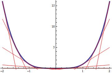
Clue to proof: any convex function can be represented as supremum of all affine functions \(a x + b\) lying below it.
Consider the simple convex function \(\phi(x)=x^2\). We deduce that if \(X\) has finite second moment then \[ (\operatorname{\mathbb{E}}\left[X|\mathcal{G}\right])^2\leq \operatorname{\mathbb{E}}\left[X^2|\mathcal{G}\right]\,.\]
Here’s a picture to illustrate the clue to the proof of Jensen’s inequality in case \(\phi(x)=x^4\):
2.10 Limits versus expectations
Often the crux of a piece of mathematics is whether one can exchange limiting operations such as \(\lim\sum\) and \(\sum\lim\). Here are a few very useful results on this, expressed in the language of expectations (the results therefore apply to both sums and integrals).
Monotone Convergence Theorem: If \(\operatorname{\mathbb{P}}\left(X_n\uparrow Y\right)=1\) and \(\operatorname{\mathbb{E}}\left[X_1\right]>-\infty\) then \[\lim_n\operatorname{\mathbb{E}}\left[X_n\right]=\operatorname{\mathbb{E}}\left[\lim_n X_n\right]=\operatorname{\mathbb{E}}\left[Y\right].\]
Note that the \(X_n\) must form an increasing sequence. We need \(\operatorname{\mathbb{E}}\left[X_1\right]>-\infty\).
Test understanding: consider case of \(X_n=-1/(nU)\) for a fixed Uniform\((0,1)\) random variable.
- Dominated Convergence Theorem: If \(\operatorname{\mathbb{P}}\left(X_n\to Y\right)=1\) and \(|X_n|\leq Z\) where \(\operatorname{\mathbb{E}}\left[Z\right]<\infty\) then \[\lim_n\operatorname{\mathbb{E}}\left[X_n\right]=\operatorname{\mathbb{E}}\left[\lim_n X_n\right]=\operatorname{\mathbb{E}}\left[Y\right].\]
Note that convergence need not be monotonic here or in the following.
Test understanding: explain why it would be enough to have finite upper and lower bounds \(\alpha\leq X_n\leq\beta\).
- Fubini’s Theorem: If \(\operatorname{\mathbb{E}}\left[|f(X,Y)|\right]<\infty\), \(X\), \(Y\) are independent, \(g(y)=\operatorname{\mathbb{E}}\left[f(X,y)\right]\), \(h(x)=\operatorname{\mathbb{E}}\left[f(x,Y)\right]\) then \[\operatorname{\mathbb{E}}\left[g(Y)\right]=\operatorname{\mathbb{E}}\left[f(X,Y)\right]=\operatorname{\mathbb{E}}\left[h(X)\right].\]
Fubini exchanges expectations rather than an expectation and a limit.
- Fatou’s lemma: If \(\operatorname{\mathbb{P}}\left(X_n\to Y\right)=1\) and \(X_n\geq0\) for all \(n\) then \[\operatorname{\mathbb{E}}\left[Y\right] \leq \lim_n \inf_{m\geq n} \operatorname{\mathbb{E}}\left[X_m\right].\]
Try Fatou if all else fails. Note that something like \(X_n\geq0\) is essential (any constant lower bound would suffice, though, it doesn’t need to be 0).