Chapter 3 Computation

Practical implementation of Bayesian methods requires substantial computation. This is required, essentially, to calculate summaries of the posterior distribution. So far, we have worked with prior distributions and likelihoods of a sufficiently convenient form to simplify the construction of the posterior. In practice,

1. we need to be able to work with much more complex models which actually relate to real life problems.

2. A “good” Bayesian will specify prior distributions that accurately reflect the prior information rather than use a prior of a mathematically convenient form.

The Bayesian needs computational tools to calculate a variety of posterior summaries from distributions that are

1. mathematically complex

2. often high-dimensional

Typically, we shall be concerned with focusing on the posterior \[\begin{eqnarray} f(\theta \, | \, x) & = & c g(\theta) \nonumber \end{eqnarray}\] where \(g(\theta) = f(x \, | \, \theta)f(\theta)\) and \(c\) is the normalising constant. In many cases \(c\) will be unknown because the integral cannot be carried out analytically.

Example 3.1 Suppose that \(X \, | \, \theta \sim N(\theta, \sigma^{2})\) where \(\sigma^{2}\) is a known constant and the prior for \(\theta\) is judged to follow a \(t\)-distribution with \(\nu\) degrees of freedom. Hence, \[\begin{eqnarray} f(\theta) & = & \frac{1}{\sqrt{\nu}B(\frac{1}{2}, \frac{1}{2} \nu)}\left(1 + \frac{\theta^{2}}{\nu}\right)^{-\frac{(\nu+1)}{2}} \nonumber \end{eqnarray}\] The posterior distribution for \(\theta \, | \, x\) is \[\begin{eqnarray} f(\theta \, | \, x) & = & \frac{c}{\sqrt{2\pi\sigma\nu}B(\frac{1}{2}, \frac{1}{2} \nu)}\left(1 + \frac{\theta^{2}}{\nu}\right)^{-\frac{(\nu+1)}{2}}\exp\left\{-\frac{1}{2\sigma^{2}}(x - \theta)^{2}\right\} \nonumber \end{eqnarray}\] where \[\begin{eqnarray} c^{-1} & = & \int_{-\infty}^{\infty} \frac{1}{\sqrt{2\pi\sigma\nu}B(\frac{1}{2}, \frac{1}{2} \nu)}\left(1 + \frac{\theta^{2}}{\nu}\right)^{-\frac{(\nu+1)}{2}}\exp\left\{-\frac{1}{2\sigma^{2}}(x - \theta)^{2}\right\} \, d\theta. \tag{3.1} \end{eqnarray}\] However, we can not perform the integral in (3.1) analytically.

In practice, many computational techniques do not explicitly require \(c\) but compute summaries of \(f(\theta \, | \, x)\) from \(g(\theta)\).

3.1 Normal approximations

We consider approximating the posterior distribution by a normal distribution. The approach utilises a Taylor series expansion of \(\log f(\theta \, | \, x)\) about the mode \(\tilde{\theta}\). The approximation is most reasonable when \(f(\theta \, | \, x)\) is unimodal and roughly symmetric.

Assume that \(\theta\) is univariate. The one-dimensional Taylor series for a generic function \(h(\theta)\) about \(\theta_{0}\) is \[\begin{eqnarray} h(\theta) & = & h(\theta_{0}) + (\theta - \theta_{0})\left.\frac{\partial}{\partial\theta} h(\theta) \right|_{\theta = \theta_{0}} + \cdots + \frac{(\theta - \theta_{0})^{r}}{r!}\left.\frac{\partial^{r}}{\partial\theta^{r}} h(\theta) \right|_{\theta = \theta_{0}} + \cdots \nonumber \end{eqnarray}\] Taking \(h(\theta) = \log f(\theta \, | \, x)\) and \(\theta_{0} = \tilde{\theta}\) we have \[\begin{eqnarray} \log f(\theta \, | \, x) & = & \log f(\tilde{\theta} \, | \, x) + (\theta - \tilde{\theta})\left.\frac{\partial}{\partial\theta}\log f(\theta \, | \, x)\right|_{\theta = \tilde{\theta}} \nonumber \\ & & + \frac{(\theta - \tilde{\theta})^{2}}{2}\left.\frac{\partial^{2}}{\partial\theta^{2}}\log f(\theta \, | \, x)\right|_{\theta = \tilde{\theta}} + \mbox{h.o.t.} \tag{3.2} \end{eqnarray}\] where h.o.t. denotes higher order terms. Now as \(\tilde{\theta}\) is the mode of \(f(\theta \, | \, x)\) then it is a maximum of \(\log f(\theta \, | \, x)\) so that \[\begin{eqnarray} \left.\frac{\partial}{\partial\theta}\log f(\theta \, | \, x)\right|_{\theta = \tilde{\theta}} & = & 0. \tag{3.3} \end{eqnarray}\] Let \[\begin{eqnarray} I(\theta \, | \, x) & = & - \frac{\partial^{2}}{\partial\theta^{2}}\log f(\theta \, | \, x) \nonumber \end{eqnarray}\] denote the observed information.

Note that as \(\tilde{\theta}\) is a maximum of \(\log f(\theta \, | \, x)\) then \(I(\tilde{\theta} \, | \, x)\) is positive.

Using \(I(\theta \, | \, x)\) and (3.3), (3.2) becomes \[\begin{eqnarray*} \log f(\theta \, | \, x) & = & \log f(\tilde{\theta} \, | \, x) - \frac{I(\tilde{\theta} \, | \, x)}{2}(\theta - \tilde{\theta})^{2} + \mbox{h.o.t.} \end{eqnarray*}\] Hence, approximately, \[\begin{eqnarray*} f(\theta \, | \, x) & \propto & \exp\left\{- \frac{I(\tilde{\theta} \, | \, x)}{2}(\theta - \tilde{\theta})^{2}\right\} \end{eqnarray*}\] which is a kernel of a \(N(\tilde{\theta}, I^{-1}(\tilde{\theta} \, | \, x))\) density so that, approximately, \(\theta \, | \, x \sim N(\tilde{\theta}, I^{-1}(\tilde{\theta} \, | \, x))\).

The approximation can be generalised for the case when \(\theta\) is multivariate. Suppose that \(\theta\) is the \(p \times 1\) vector \((\theta_{1}, \ldots, \theta_{p})^{T}\) with posterior density \(f(\theta \, | \, x)\). Let the posterior mode be \(\tilde{\theta} = (\tilde{\theta}_{1}, \ldots, \tilde{\theta}_{p})^{T}\) and the \(p \times p\) observed information matrix be \(I(\theta \, | \, x)\) where \[\begin{eqnarray} (I(\theta \, | \, x))_{ij} - \frac{\partial^{2}}{\partial\theta_{i}\partial\theta_{j}}\log f(\theta \, | \, x) \nonumber \end{eqnarray}\] then, approximately, \(\theta \, | \, x \sim N_{p}(\tilde{\theta}, I^{-1}(\tilde{\theta} \, | \, x))\), the multivariate normal distribution (of dimension \(p\)) with \[\begin{eqnarray} f(\theta \, | \, x) & = & \frac{1}{(2 \pi)^{\frac{p}{2}} |I^{-1}(\tilde{\theta} \, | \, x)|^{\frac{1}{2}}} \exp\left\{-\frac{1}{2} (\theta - \tilde{\theta})^{T} I^{-1}(\tilde{\theta} \, | \, x) (\theta - \tilde{\theta})\right\}. \nonumber \end{eqnarray}\]

Example 3.2 Suppose that \(X_{1}, \ldots, X_{n}\) are exchangeable and \(X_{i} \, | \, \theta \sim Po(\theta)\). Find a Normal approximation to the posterior distribution when we judge a uniform (improper) prior is appropriate for \(\theta\).

We take \(f(\theta) \propto 1\) so that \[\begin{eqnarray} f(\theta \, | \, x) & \propto & \prod_{i=1}^{n} \theta^{x_{i}} e^{-\theta} \nonumber \ = \ \theta^{n\bar{x}}e^{-n\theta} \nonumber \end{eqnarray}\] which we recognise as a kernel of a \(Gamma(n\bar{x} + 1, n)\) distribution thus \(\theta \, | \, x \sim Gamma(n\bar{x} + 1, n)\). A \(Gamma(\alpha, \beta)\) distribution has mode equal to \(\frac{\alpha - 1}{\beta}\) so that the mode of \(\theta \, | \, x\) is \(\tilde{\theta} = \frac{n\bar{x} + 1 - 1}{n} = \bar{x}\). The observed information is \[\begin{eqnarray} I(\theta \, | \, x) \ = \ - \frac{\partial^{2}}{\partial\theta^{2}}\left\{n\bar{x} \log \theta - n \theta + \log \frac{n^{n\bar{x}+1}}{\Gamma(n\bar{x}+1)}\right\} \ = \ \frac{n\bar{x}}{\theta^{2}} \nonumber \end{eqnarray}\] so that \(I(\tilde{\theta} \, | \, x) = I(\bar{x} \, | \, x) = \frac{n}{\bar{x}}\). Thus, approximately, \(\theta \, | \, x \sim N(\bar{x}, \frac{\bar{x}}{n})\).

3.2 Posterior sampling

If we can draw a sample of values from the posterior distribution then we can use the properties of the sample (e.g. mean, variance, quantiles, \(\ldots\)) to estimate properties of the posterior distribution.

3.2.1 Monte Carlo integration

Suppose that we wish to estimate \(E\{g(X)\}\) for some function \(g(x)\) with respect to a density \(f(x)\). Thus, \[\begin{eqnarray} E\{g(X)\} & = & \int_{X} g(x)f(x) \, dx. \tag{3.4} \end{eqnarray}\] For example, to compute the posterior mean of \(\theta \, | \, x\) we have \[\begin{eqnarray} E(\theta \, | \, X) & = & \int_{\theta} \theta f(\theta \, | \, x) \, d\theta. \nonumber \end{eqnarray}\]

The term Monte Carlo was introduced by John von Neumann (1903-1957) and Stanislaw Ulam (1909-1984) as a code word for the simulation work they were doing for the Manhattan Project during World War II.

Monte Carlo integration involves the following:

1. sample \(N\) values \(x_{1}, \ldots, x_{N}\) independently from \(f(x)\)

We shall later see how obtaining an independent sample can be difficult.

2. calculate \(g(x_{i})\) for each \(x_{i}\)

3. estimate \(E\{g(X)\}\) by the sample mean of the \(g(x_{i})\), \[\begin{eqnarray} g_{N}(x) & = & \frac{1}{N} \sum_{i=1}^{N} g(x_{i}). \nonumber \end{eqnarray}\] Note that the corresponding estimator \(g_{N}(X)\) is an unbiased estimator of \(E\{g(X)\}\) as \[\begin{eqnarray} E\{g_{N}(X)\} & = & \frac{1}{N} \sum_{i=1}^{N} E\{g(X_{i})\} \nonumber \\ & = & \sum_{i=1}^{N} E\{g(X)\} \ = \ E\{g(X)\}. \nonumber \end{eqnarray}\] The variance of the estimator is \[\begin{eqnarray} Var\{g_{N}(X)\} & = & \frac{1}{N^{2}} \sum_{i=1}^{N} Var\{g(X_{i})\} \nonumber \\ & = & \frac{1}{N^{2}} \sum_{i=1}^{N} Var\{g(X)\} \ = \ \frac{1}{N}Var\{g(X)\}.\nonumber \end{eqnarray}\]

3.2.2 Importance sampling

Suppose that we can not sample from \(f(x)\) but can generate samples from some other distribution \(q(x)\) which is an approximation to \(f(x)\).

e.g. \(q(x)\) might be the approximation to \(f(x)\) obtained by a Normal approximation about the mode.

We can use samples from \(q(x)\) using the method of importance sampling. Let us consider the problem of estimating \(E\{g(X)\}\) for some function \(g(x)\) with respect to a density \(f(x)\). Then we may rewrite (3.4) as \[\begin{eqnarray} E\{g(X)\} & = & \int_{X} \frac{g(x)f(x)}{q(x)}q(x) \, dx \nonumber \\ & = & E\left.\left\{\frac{g(X)f(X)}{q(X)} \, \right| \, X \sim q(x) \right\} \tag{3.5} \end{eqnarray}\] where (3.5) makes clear that the expectation is calculation with respect to the density \(q(x)\). If we draw a random sample \(x_{1}, \ldots, x_{N}\) from \(q(x)\) then we may approximate \(E\{g(X)\}\) by \[\begin{eqnarray*} \hat{I} & = & \frac{1}{N} \sum_{i=1}^{N} \frac{g(x_{i})f(x_{i})}{q(x_{i})}. \end{eqnarray*}\] Notice that \[\begin{eqnarray*} E(\hat{I} \, | \, X \sim q(x) ) & = & \frac{1}{N} \sum_{i=1}^{N} E\left.\left(\frac{g(X_{i})f(X_{i})}{q(X_{i})} \, \right| \, X \sim q(x) \right) \\ & = & \frac{1}{N} \sum_{i=1}^{N} E\left.\left(\frac{g(X)f(X)}{q(X)} \, \right| \, X \sim q(x) \right) \ = \ E\{g(X)\} \end{eqnarray*}\] so that \(\hat{I}\) is an unbiased estimator of \(E\{g(X)\}\). In a similar fashion we obtain that \[\begin{eqnarray*} Var(\hat{I} \, | \, X \sim q(x) ) & = & \frac{1}{N} Var\left.\left(\frac{g(X)f(X)}{q(X)} \, \right| \, X \sim q(x) \right). \end{eqnarray*}\] Hence, the variance of \(\hat{I}\) will depend both on the choice of \(N\) and the approximation \(q(x)\). Given a choice of approximating distributions from which we can sample we might choose the approximation which minimises the variance of \(\hat{I}\).

3.3 Markov chain Monte Carlo (MCMC)

Markov chain Monte Carlo (MCMC) is a general technique that has revolutionised practical Bayesian statistics. It is a tool that generates samples from complex multi-dimensional posterior distributions in cases where the distribution is analytically intractable.

A Markov chain is a random process with the property that, conditional upon its current value, future values are independent of the past. Under certain conditions such a chain will converge to a stationary distribution so that eventually values may be treated as a sample from the stationary distribution.

The basic idea behind MCMC techniques for Bayesian statistics is:

1. Construct a Markov chain that has the required posterior distribution as its stationary distribution. This is sometimes referred to as the target distribution.

2. From some starting point, generate sequential values from the chain until (approximate) convergence. (One of the difficulties of the approach is knowing when this has occurred.)

3. Continue generating values from the chain which are now viewed as a sample of values from the posterior distribution. (As the chain has converged, we are now sampling from the stationary distribution.)

4. Use the resulting sample (from the stationary distribution) to estimate properties of the posterior distribution.

3.3.1 Useful results for Markov chains

We will consider only discrete time Markov chains (simulation is itself discrete) and summarise only the important definitions required for MCMC.

A Markov chain is a discrete time stochastic process \(\{X_{0}, X_{1}, \ldots\}\) with the property that the distribution of \(X_{t}\) given all previous values of the process only depends upon \(X_{t-1}\). That is, \[\begin{eqnarray} P(X_{t} \in A \, | \, X_{0} = x_{0}, X_{1} = x_{1}, \ldots, X_{t-1} = x_{t-1}) & = & P(X_{t} \in A \, | \, X_{t-1} = x_{t-1}) \nonumber \end{eqnarray}\] for any set \(A\).

The probability of a transition, or jump, from \(x_{t-1}\) at time \(t-1\) to \(X_{t}\) at time \(t\) is given by the transition kernel. If \(X_{t}\) is discrete then the transition kernel is a transition matrix with \((i, j)\)th element \[\begin{eqnarray} P_{ij} & = & P(X_{t} = j \, | \, X_{t-1} = i) \tag{3.6} \end{eqnarray}\] which represents the probability of moving from state \(i\) to state \(j\). In the continuous case, if \[\begin{eqnarray} P(X_{t} \in A \, | \, X_{t-1} = x_{t-1}) & = & \int_{A} q(x \, | \, x_{t-1}) \, dx \tag{3.7} \end{eqnarray}\] then the transition kernel is \(q(x \, | \, x_{t-1})\). Notice that it is common to see the transition kernel written as \(q(x_{t-1}, x)\) to indicate the transition from \(x_{t-1}\) to \(x\); \(q(x_{t-1}, x)\) does not represent the joint density of \(x_{t-1}\) and \(x\).

Definition 3.1 (Irreducible) A Markov chain is said to be irreducible if for every \(i\), \(j\) there exists \(k\) such that \[\begin{eqnarray} P(X_{t+k} = j \, | \, X_{t} = i) & > & 0 \nonumber \end{eqnarray}\] that is, all states can be reached from any other state in a finite number of moves.

Definition 3.2 (Periodic/Aperiodic) A state \(i\) is said to be periodic with period \(d_{i}\) if starting from state \(i\) the chain returns to it within a fixed number of steps \(d_{i}\) or a multiple of \(d_{i}\). \[\begin{eqnarray} d_{i} & = & \mbox{gcd} \{t : P(X_{t} = i \, | \, X_{0} = i) > 0\} \nonumber \end{eqnarray}\] where \(\mbox{gcd}\) is the greatest common divisor. If \(d_{i} = 1\) then the state \(i\) is said to be aperiodic.

Irreducible Markov chains have the property that all states have the same period. A Markov chain is called aperiodic if some (and hence all) states are aperiodic.

Definition 3.3 (Recurrent/Positive Recurrent) Let \(\tau_{ii}\) be the time of the first return to state \(i\) \[\begin{eqnarray} t_{ii} & = & \min\{t > 0: X_{t} = i \, | \, X_{0} = i\} \nonumber \end{eqnarray}\] A state \(i\) is recurrent if \(P(\tau_{ii} < \infty) = 1\) and positive recurrent if \(E(\tau_{ii}) < \infty\).

Thus, a state \(i\) is recurrent if the chain will return to state \(i\) with probability 1 and positive recurrent if, with probability 1, it will return in a finite time. An irreducible Markov chain is positive recurrent if some (and hence all) states \(i\) are positive recurrent.

Definition 3.4 (Ergodic) A state is said to be ergodic if it is aperiodic and positive recurrent. A Markov chain is ergodic if all of its states are ergodic.

Definition 3.5 (Stationary) A distribution \(\pi\) is said to be a stationary distribution of a Markov chain with transition probabilities \(P_{ij}\), see (3.6), if \[\begin{eqnarray} \sum_{i \in S} \pi_{i} P_{ij} & = & \pi_{j} \ \ \forall j \in S \nonumber \end{eqnarray}\] where \(S\) denotes the state space.

In matrix notation if \(P\) is the matrix of transition probabilities and \(\pi\) the vector with \(i\)th entry \(\pi_{i}\) then the stationary distribution satisfies \[\begin{eqnarray*} \pi & = & \pi P \end{eqnarray*}\] These definitions have assumed that the state space of the chain is discrete. They are naturally generalised to the case when the state space is continuous. For example if \(q(x \, | \, x_{t-1})\) denotes the transition kernel, see (3.7), then the stationary distribution \(\pi\) of the Markov chain must satisfy \[\begin{eqnarray*} \pi(x) & = & \int \pi(x_{t-1})q(x \, | \, x_{t-1}) \, dx_{t-1} \end{eqnarray*}\]

Theorem 3.1 (Existence and uniqueness) Each irreducible and aperiodic Markov chain has a unique stationary distribution \(\pi\).

Theorem 3.2 (Convergence) Let \(X_{t}\) be an irreducible and aperiodic Markov chain with stationary distribution \(\pi\) and arbitrary initial value \(X_{0} = x_{0}\). Then \[\begin{eqnarray} P(X_{t} = x \, | \, X_{0} = x_{0}) & \rightarrow & \pi(x) \nonumber \end{eqnarray}\] as \(t \rightarrow \infty\).

Theorem 3.3 (Ergodic) Let \(X_{t}\) be an ergodic Markov chain with limiting distribution \(\pi\). If \(E\{g(X) \, | \, X \sim \pi(x)\} < \infty\) then the sample mean converges to the expectation of \(g(X)\) under \(\pi\), \[\begin{eqnarray} P\left\{\frac{1}{N} \sum_{i=1}^{N} g(X_{i}) \rightarrow E\{g(X) \, | \, X \sim \pi(x)\}\right\} & = & 1. \nonumber \end{eqnarray}\]

Consequence of these theorems:

If we can construct an ergodic Markov chain \(\theta_{t}\) which has the posterior distribution \(f(\theta \, | \, x)\) as the stationary distribution \(\pi(\theta)\) then, starting from an initial point \(\theta_{0}\), if we run the Markov chain for long enough, we will sample from the posterior.

1. for large \(t\), \(\theta_{t} \sim \pi(\theta) = f(\theta \, | \, x)\)

2. for each \(s > t\), \(\theta_{s} \sim \pi(\theta) = f(\theta \, | \, x)\)

3. the ergodic averages converge to the desired expectations under the target distribution.

3.3.2 The Metropolis-Hastings algorithm

Suppose that our goal is to draw samples from some distribution \(f(\theta \, | \, x) = cg(\theta)\) where \(c\) is the normalising constant which may not be known or very difficult to compute.

The original algorithm was developed by Nicholas Metropolis (1915-1999) in 1953 and generalised by W. Keith Hastings (1930-2016) in 1970. Metropolis, aided by the likes of Mary Tsingou (1928-) and Klara Dan von Neumann (1911-1963), was involved in the design and build of the MANIAC I computer.

The Metropolis-Hastings algorithm provides a way of sampling from \(f(\theta \, | \, x)\) without requiring us to know \(c\).

The algorithm can be used to sample from any distribution \(f(\theta)\). In this course, our interest centres upon sampling from the posterior distribution.

Let \(q(\phi \, | \, \theta)\) be an arbitrary transition kernel: that is the probability of moving, or jumping, from current state \(\theta\) to proposed new state \(\phi\), see (3.7). This is sometimes called the proposal distribution. The following algorithm will generate a sequence of values \(\theta^{(1)}\), \(\theta^{(2)}\), \(\ldots\) which form a Markov chain with stationary distribution given by \(f(\theta \, | \, x)\).

The Metropolis-Hastings Algorithm.

1. Choose an arbitrary starting point \(\theta^{(0)}\) for which \(f(\theta^{(0)} \, | \, x) > 0\).

2. At time t

   1. Sample a candidate point or proposal, \(\theta^{*}\), from \(q(\theta^{*} \, | \, \theta^{(t-1)})\), the proposal distribution.

   2. Calculate the acceptance probability \[\begin{eqnarray} \alpha(\theta^{(t-1)}, \theta^{*}) & = & \min \left(1, \frac{f(\theta^{*} \, | \, x)q(\theta^{(t-1)} \, | \, \theta^{*})}{f(\theta^{(t-1)} \, | \, x)q(\theta^{*} \, | \, \theta^{(t-1)})} \right). \tag{3.8} \end{eqnarray}\]

   3. Generate \(U \sim U(0, 1)\).

   4. If \(U \leq \alpha(\theta^{(t-1)}, \theta^{*})\) accept the proposal and set \(\theta^{(t)} = \theta^{*}\). Otherwise, reject the proposal and set \(\theta^{(t)} = \theta^{(t-1)}\). (We thus accept the proposal with probability \(\alpha(\theta^{(t-1)}, \theta^{*})\).)

3. Repeat step 2.

Notice that if \(f(\theta \, | \, x) = cg(\theta)\) then, from (3.8), \[\begin{eqnarray} \alpha(\theta^{(t-1)}, \theta^{*}) & = & \min \left(1, \frac{cg(\theta^{*})q(\theta^{(t-1)} \, | \, \theta^{*})}{cg(\theta^{(t-1)})q(\theta^{*} \, | \, \theta^{(t-1)})} \right) \nonumber \\ & = & \min \left(1, \frac{g(\theta^{*})q(\theta^{(t-1)} \, | \, \theta^{*})}{g(\theta^{(t-1)})q(\theta^{*} \, | \, \theta^{(t-1)})} \right) \nonumber \end{eqnarray}\] so that we do not need to know the value of \(c\) in order to compute \(\alpha(\theta^{(t-1)}, \theta^{*})\) and hence utilise the Metropolis-Hastings algorithm to sample from \(f(\theta \, | \, x)\).

If the proposal distribution is symmetric, so \(q(\phi \, | \, \theta) = q(\theta \, | \, \phi)\) for all possible \(\phi\), \(\theta\), then, in particular, we have \(q(\theta^{(t-1)} \, | \, \theta^{*}) = q(\theta^{*} \, | \, \theta^{(t-1)})\) so that the acceptance probability (3.8) is given by \[\begin{eqnarray} \alpha(\theta^{(t-1)}, \theta^{*}) & = & \min \left(1, \frac{f(\theta^{*} \, | \, x)}{f(\theta^{(t-1)} \, | \, x)} \right). \tag{3.9} \end{eqnarray}\] The Metropolis-Hastings algorithm with acceptance probability (3.8) replaced by (3.9) is the Metropolis algorithm and was the initial version of this MCMC approach before later being generalised by Hastings. In this context it is straightforward to interpret the acceptance/rejection rule.

1. If the proposal increases the posterior density, that is \(f(\theta^{*} \, | \, x) > f(\theta^{(t-1)} \, | \, x)\), we always move to the new point \(\theta^{*}\).

2. If the proposal decreases the posterior density, that is \(f(\theta^{*} \, | \, x) < f(\theta^{(t-1)} \, | \, x)\), then we move to the new point \(\theta^{*}\) with probability equal to the ratio of the new to current posterior density.

Example 3.3 Suppose that we want to sample from \(\theta \, | \, x \sim N(0, 1)\) using the Metropolis-Hastings algorithm and we let the proposal distribution \(q(\phi \, | \, \theta)\) be the density of the \(N(\theta, \sigma^{2})\) for some \(\sigma^{2}\). Thus, \[\begin{eqnarray} q(\phi \, | \, \theta) & = & \frac{1}{\sqrt{2\pi}\sigma} \exp \left\{-\frac{1}{2\sigma^{2}}(\phi - \theta)^{2}\right\} \nonumber \\ & = & \frac{1}{\sqrt{2\pi}\sigma} \exp \left\{-\frac{1}{2\sigma^{2}}(\theta - \phi)^{2}\right\} \nonumber \\ & = & q(\theta \, | \, \phi). \nonumber \end{eqnarray}\] The proposal distribution is symmetric and so the Metropolis-Hastings algorithm reduces to the Metropolis algorithm. The algorithm is performed as follows.

1. Choose a starting point \(\theta^{(0)}\) for which \(f(\theta^{(0)} \, | \, x) > 0\). As \(\theta \, | \, x \sim N(0, 1)\) this will hold for any \(\theta^{(0)} \in (-\infty, \infty)\).

2. At time \(t\)

   1. Sample \(\theta^{*} \sim N(\theta^{(t-1)}, \sigma^{2})\).

   2. Calculate the acceptance probability \[\begin{eqnarray} \alpha(\theta^{(t-1)}, \theta^{*}) & = & \min \left(1, \frac{f(\theta^{*} \, | \, x)}{f(\theta^{(t-1)} \, | \, x)} \right) \nonumber \\ & = & \min \left(1, \frac{(2\pi)^{-\frac{1}{2}} \exp\{-\frac{1}{2}(\theta^{*})^{2}\}}{(2\pi)^{-\frac{1}{2}} \exp\{-\frac{1}{2}(\theta^{(t-1)})^{2}\}}\right). \nonumber \end{eqnarray}\]

   3. Generate \(U \sim U(0, 1)\).

   4. If \(U \leq \alpha(\theta^{(t-1)}, \theta^{*})\) accept the move, \(\theta^{(t)} = \theta^{*}\). Otherwise reject the move, \(\theta^{(t)} = \theta^{(t-1)}\).

3. Repeat step 2.

Example 3.4 We shall now illustrate the results of Example 3.3 using a simulation exercise in R. The function metropolis (courtesy of Ruth Salway) uses the Metropolis-Hastings algorithm to sample from \(N(\mbox{mu.p}, \mbox{sig.p}^{2})\) with the proposal \(N(\mbox{theta[t-1]},\mbox{sig.q}^{2})\).

metropolis = function (start=1, n=100, sig.q=1, mu.p=0, sig.p=1) {

#starting value theta_0 = start
#run for n iterations

  #set up vector theta[] for the samples
  theta=rep(NA,n)
  theta[1]=start

  #count the number of accepted proposals
  accept=0

  #Main loop
  for (t in 2:n) {

    #pick a candidate value theta* from N(theta[t-1], sig.q)
    theta.star = rnorm(1, theta[t-1], sqrt(sig.q))
    
    #generate a random number between 0 and 1:
    u = runif(1)

    # calculate acceptance probability:
    r = (dnorm(theta.star,mu.p,sig.p)) / (dnorm(theta[t-1],mu.p,sig.p) )
    
    a=min(r,1)
    
    #if u<a we accept the proposal; otherwise we reject
    if (u<a) {   
        #accept
            accept=accept+1
            theta[t] = theta.star
    }
    else {
        #reject
        theta[t] = theta[t-1]
        }
  #end loop
  }
}  

We illustrate two example runs from of the algorithm. Firstly, in Figures 3.1 - 3.3, for \(\theta \, | \, x \sim N(0, 1)\) where the proposal distribution is normal with mean \(\theta\) and chosen variance \(\sigma^{2} = 1\) and the starting point is \(\theta^{(0)} = 1\) and secondly, in Figures 3.4 - 3.6, for \(\theta \, | \, x \sim N(0, 1)\) where the proposal distribution is normal with mean \(\theta\) and chosen variance \(\sigma^{2} = 0.36\) and the starting point is \(\theta^{(0)} = 1\). In each case we look at the results for nine, 100 and 5000 iterations from the sampler.

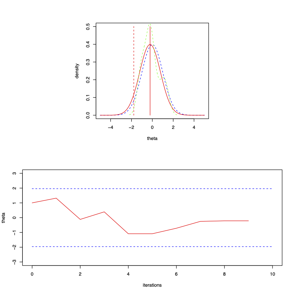
Figure 3.1: Nine iterations from a Metropolis-Hastings sampler for \(\theta | x \sim N(0, 1)\) where the proposal distribution is normal with mean \(\theta\) and chosen variance \(\sigma^{2} = 1\) and the starting point is \(\theta^{(0)} = 1\). The top plot shows the target distribution, \(N(0, 1)\), the proposal distribution for \(\theta^{(9)}\) which is \(N(-0.216, 1)\), the proposal \(\theta^{*} = -1.779\) and the current observed density. The move is rejected; the bottom plot is the trace plot of \(\theta^{(t)}\).

The following table summarises the stages of the algorithm for the iterations given in Figure 3.1. \[\begin{eqnarray} \begin{array}{c|r|c|r} t & \theta^{*} & \mbox{Accept/Reject?} & \theta^{(t)} \\ \hline 1 & 1.319 & \mbox{Accept} & 1.319 \\ 2 & -0.118 & \mbox{Accept} & -0.118 \\ 3 & 0.392 & \mbox{Accept} & 0.392 \\ 4 & -1.089 & \mbox{Accept} & -1.089 \\ 5 & -1.947 & \mbox{Reject} & -1.089 \\ 6 & -0.716 & \mbox{Accept} & -0.716 \\ 7 & -0.251 & \mbox{Accept} & -0.251 \\ 8 & -0.216 & \mbox{Accept} & -0.216 \\ 9 & -1.779 & \mbox{Reject} & -0.216 \end{array} \nonumber \end{eqnarray}\]

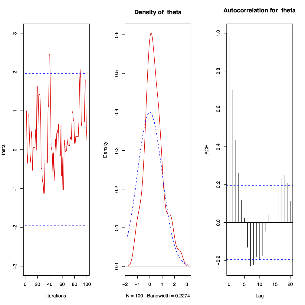
Figure 3.2: 100 iterations from a Metropolis-Hastings sampler for \(\theta | x \sim N(0, 1)\) where the proposal distribution is normal with mean \(\theta\) and chosen variance \(\sigma^{2} = 1\) and the starting point is \(\theta^{(0)} = 1\). The first plot shows the trace plot of \(\theta^{(t)}\), the second the observed density against the target density and the third the autocorrelation plot. The sample mean is \(0.3435006\) and the sample variance is \(0.5720027\). 3% of points were observed to be greater than \(1.96\) and the acceptance rate is \(0.66\).

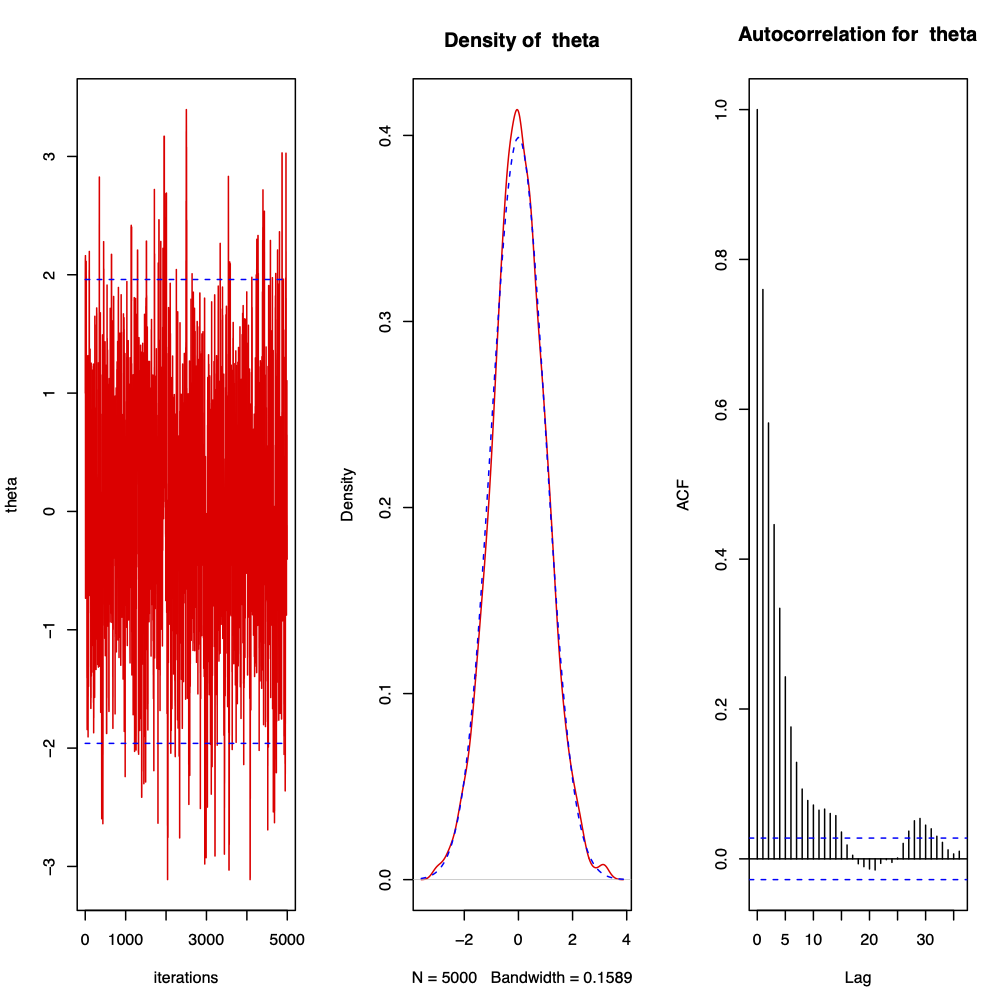
Figure 3.3: 5000 iterations from a Metropolis-Hastings sampler for \(\theta | x \sim N(0, 1)\) where the proposal distribution is normal with mean \(\theta\) and chosen variance \(\sigma^{2} = 1\) and the starting point is \(\theta^{(0)} = 1\). The first plot shows the trace plot of \(\theta^{(t)}\), the second the observed density against the target density and the third the autocorrelation plot. The sample mean is \(0.01340934\) and the sample variance is \(0.984014\). 2.76% of points were observed to be greater than \(1.96\) and the acceptance rate is \(0.7038\).

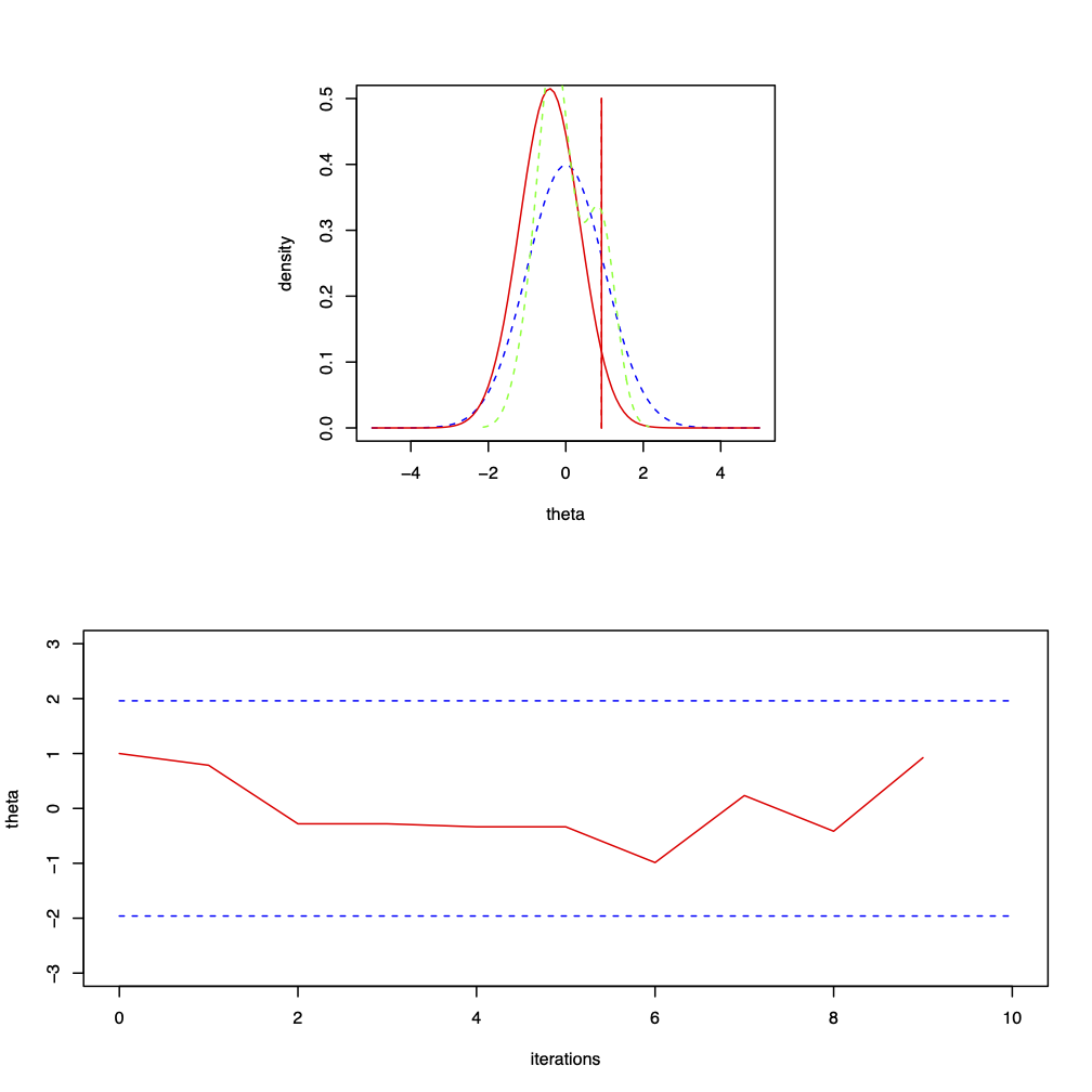
Figure 3.4: Nine iterations from a Metropolis-Hastings sampler for \(\theta | x \sim N(0, 1)\) where the proposal distribution is normal with mean \(\theta\) and chosen variance \(\sigma^{2} = 0.36\) and the starting point is \(\theta^{(0)} = 1\). The top plot shows the target distribution, \(N(0, 1)\), the proposal distribution for \(\theta^{(9)}\) which is \(N(-0.416, 0.36)\), the proposal \(\theta^{*} = 0.923\) and the current observed density. The move is accepted; the bottom plot is the trace plot of \(\theta^{(t)}\).

The following table summarises the stages of the algorithm for the iterations given in Figure 3.4. \[\begin{eqnarray} \begin{array}{c|r|c|r} t & \theta^{*} & \mbox{Accept/Reject?} & \theta^{(t)} \\ \hline 1 & 0.786 & \mbox{Accept} & 0.786 \\ 2 & -0.280 & \mbox{Accept} & -0.280 \\ 3 & -1.092 & \mbox{Reject} & -0.280 \\ 4 & -0.335 & \mbox{Accept} & -0.335 \\ 5 & -1.169 & \mbox{Reject} & -0.335 \\ 6 & -0.987 & \mbox{Accept} & -0.987 \\ 7 & 0.234 & \mbox{Accept} & 0.234 \\ 8 & -0.416 & \mbox{Accept} & -0.416 \\ 9 & 0.923 & \mbox{Reject} & 0.923 \end{array} \nonumber \end{eqnarray}\]

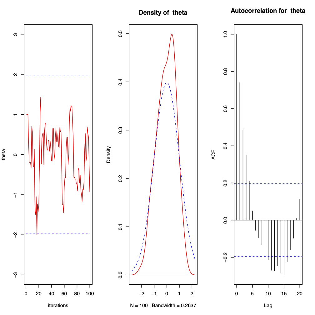
Figure 3.5: 100 iterations from a Metropolis-Hastings sampler for \(\theta | x \sim N(0, 1)\) where the proposal distribution is normal with mean \(\theta\) and chosen variance \(\sigma^{2} = 0.36\) and the starting point is \(\theta^{(0)} = 1\). The first plot shows the trace plot of \(\theta^{(t)}\), the second the observed density against the target density and the third the autocorrelation plot. The sample mean is \(-0.04438661\) and the sample variance is \(0.5414882\). 0% of points were observed to be greater than \(1.96\) and the acceptance rate is \(0.83\).

Notice that, by comparing Figure 3.5 with Figure 3.2, reducing \(\sigma^{2}\), that is we are proposing smaller jumps, increases the acceptance rate but reduces the mixing.

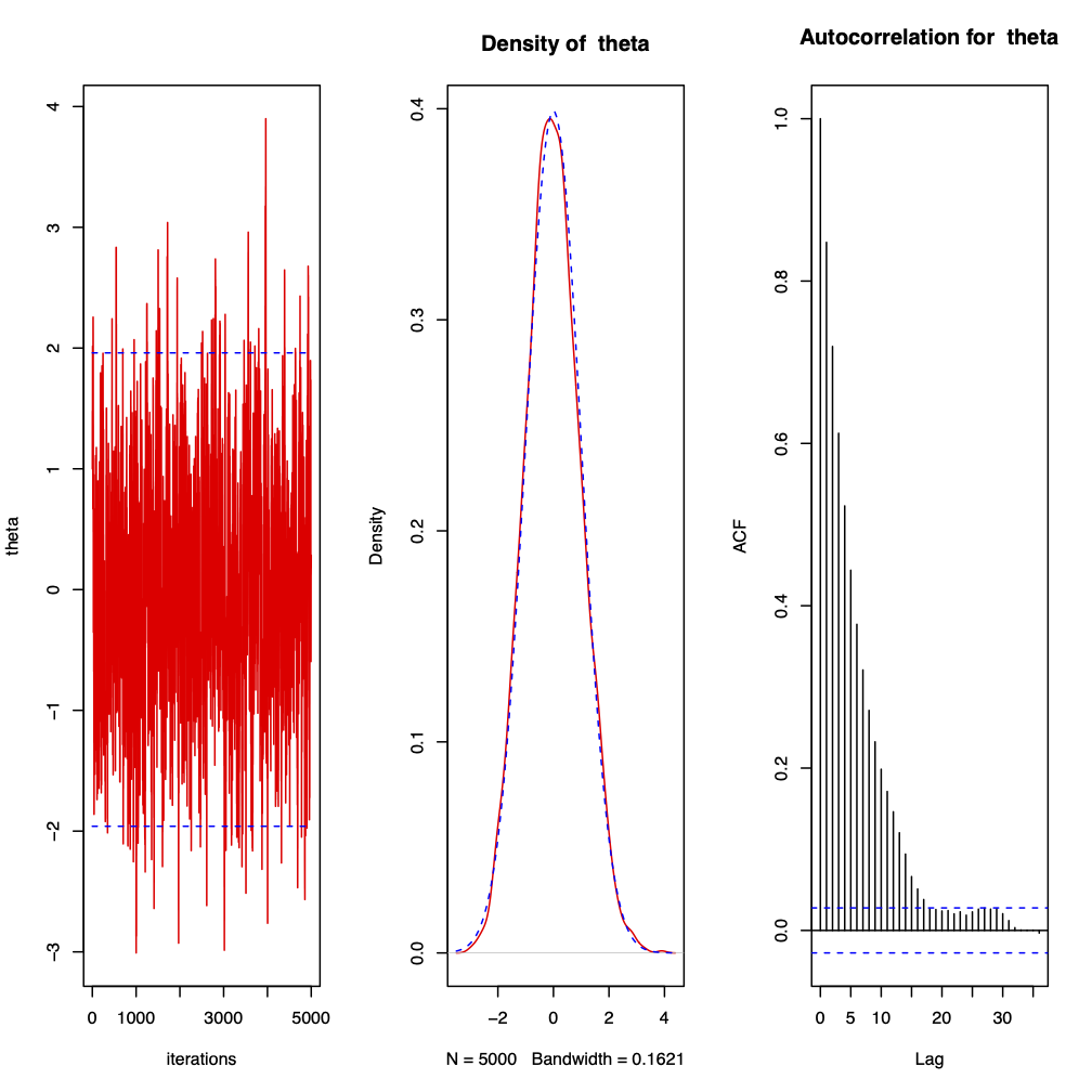
Figure 3.6: 5000 iterations from a Metropolis-Hastings sampler for \(\theta | x \sim N(0, 1)\) where the proposal distribution is normal with mean \(\theta\) and chosen variance \(\sigma^{2} = 0.36\) and the starting point is \(\theta^{(0)} = 1\). The first plot shows the trace plot of \(\theta^{(t)}\), the second the observed density against the target density and the third the autocorrelation plot. The sample mean is \(-0.008158827\) and the sample variance is \(0.9792388\). 2.42% of points were observed to be greater than \(1.96\) and the acceptance rate is \(0.7894\).

3.3.3 Gibbs sampler

The aim of the Gibbs sampler is to make sampling from a high-dimensional distribution more tractable by sampling from a collection of more manageable smaller dimensional distributions.

Josiah Willard Gibbs (1839-1903)

Gibbs sampling is a MCMC scheme where the transition kernel is formed by the full conditional distributions. Assume that the distribution of interest is \(\pi(\theta)\) where \(\theta = (\theta_{1}, \ldots, \theta_{d})\). Note that

1. Typically we will want \(\pi(\theta) = f(\theta \, | \, x)\).

2. The components \(\theta_{i}\) can be a scalar, a vector or a matrix. For simplicity of exposition you may regard them as scalars.

Let \(\theta_{-i}\) denote the set \(\theta \setminus \theta_{i}\) and suppose that the full conditional distributions \(\pi_{i}(\theta_{i}) = \pi(\theta_{i} \, | \, \theta_{-i})\) \(i = 1, \ldots, d\) are available and can be sampled from.

The Gibbs sampler

1. Choose an arbitrary starting point \(\theta^{(0)} = (\theta^{(0)}_{1}, \ldots, \theta^{(0)}_{d})\) for which \(\pi(\theta^{(0)}) > 0\).

2. • Obtain \(\theta_{1}^{(t)}\) from conditional distribution \(\pi(\theta_{1} \, | \, \theta_{2}^{(t-1)}, \ldots, \theta_{d}^{(t-1)})\)

   • Obtain \(\theta_{2}^{(t)}\) from conditional distribution \(\pi(\theta_{2} \, | \, \theta_{1}^{(t)}, \theta_{3}^{(t-1)}, \ldots, \theta_{d}^{(t-1)})\) \[\begin{eqnarray} & \vdots & \nonumber \end{eqnarray}\]

   • Obtain \(\theta_{p}^{(t)}\) from conditional distribution \(\pi(\theta_{p} \, | \, \theta_{1}^{(t)}, \ldots, \theta_{p-1}^{(t)}, \theta_{p+1}^{(t-1)}, \ldots, \theta_{d}^{(t-1)})\) \[\begin{eqnarray} & \vdots & \nonumber \end{eqnarray}\]

   • Obtain \(\theta_{d}^{(t)}\) from conditional distribution \(\pi(\theta_{d} \, | \, \theta_{1}^{(t)}, \ldots, \theta_{d-1}^{(t)})\)

3. Repeat step 2.

The algorithm is run until convergence is reached.

We’ll look at more detail into strategies for judging this in a couple of lectures time.

When convergence is reached, the resulting value \(\theta^{(j)}\) is a realisation (or draw) from \(\pi(\theta)\).

Example 3.5 Suppose that the joint distribution of \(\theta = (\theta_{1}, \theta_{2})\) is given by \[\begin{eqnarray} f(\theta_{1}, \theta_{2}) & \propto & \binom{n}{\theta_{1}} \theta_{2}^{\theta_{1} + \alpha - 1}(1-\theta_{2})^{n-\theta_{1}+\beta-1} \nonumber \end{eqnarray}\] for \(\theta_{1} \in [0, 1, \ldots, n]\) and \(0 \leq \theta_{2} \leq 1\). Hence, \(\theta_{1}\) is discrete and \(\theta_{2}\) is continuous. Suppose that we are interested in calculating some characteristic of the marginal distribution of \(\theta_{1}\). The Gibbs sampler will allow us to generate a sample from this marginal distribution in the following way.

The conditional distributions are \[\begin{eqnarray} \theta_{1} \, | \, \theta_{2} & \sim & Bin(n, \theta_{2}) \nonumber \\ \theta_{2} \, | \, \theta_{1} & \sim & Beta(\theta_{1} + \alpha, n - \theta_{1} + \beta) \nonumber \end{eqnarray}\] Assuming the hyperparameters \(n\), \(\alpha\) and \(\beta\) are known then it is straightforward to sample from these distributions and we now generate a “Gibbs sequence” of random variables.

• Step 1: Specify an initial value \(\theta_{1}^{(0)}\) and either specify an initial \(\theta_{2}^{(0)}\) or sample it from \(\pi(\theta_{2} \, | \, \theta_{1}^{(0)})\), the \(Beta(\theta_{1}^{(0)} + \alpha, n - \theta_{1}^{(0)} + \beta)\) distribution, to obtain \(\theta_{2}^{(0)}\).

• Step 2.1.(a): Obtain \(\theta_{1}^{(1)}\) from sampling from \(\pi(\theta_{1} \, | \, \theta_{2}^{(0)})\), the \(Bin(n, \theta_{2}^{(0)})\) distribution.

• Step 2.1.(b): Obtain \(\theta_{2}^{(1)}\) from sampling from \(\pi(\theta_{2} \, | \, \theta_{1}^{(1)})\), the \(Beta(\theta_{1}^{(1)} + \alpha, n - \theta_{1}^{(1)} + \beta)\) distribution.

• Step 2.2.(a): Obtain \(\theta_{1}^{(2)}\) from sampling from \(\pi(\theta_{1} \, | \, \theta_{2}^{(1)})\), the \(Bin(n, \theta_{2}^{(1)})\) distribution.

• Step 2.2.(b): Obtain \(\theta_{2}^{(2)}\) from sampling from \(\pi(\theta_{2} \, | \, \theta_{1}^{(2)})\), the \(Beta(\theta_{1}^{(2)} + \alpha, n - \theta_{1}^{(2)} + \beta)\) distribution.

We continue to run through the algorithm to obtain the sequence of values \[\begin{eqnarray} \theta_{1}^{(0)}, \, \theta_{2}^{(0)}, \, \theta_{1}^{(1)}, \, \theta_{2}^{(1)}, \, \theta_{1}^{(2)}, \, \theta_{2}^{(2)}, \ldots, \, \theta_{1}^{(k)}, \, \theta_{2}^{(k)} \nonumber \end{eqnarray}\] which may be expressed as \(\theta^{(0)}, \, \theta^{(1)}, \, \theta^{(2)}, \ldots, \, \theta^{(k)}\) where \(\theta^{(t)} = (\theta_{1}^{(t)}, \theta_{2}^{(t)})\). The sequence is such that the distribution of \(\theta_{1}^{(k)}\) tends to \(f(\theta_{1})\) as \(k \rightarrow \infty\) and, similarly, the distribution of \(\theta_{2}^{(k)}\) tends to \(f(\theta_{2})\) as \(k \rightarrow \infty\).

To allow the sequence to converge to the stationary distribution, we first remove what are termed the “burn-in” samples. Suppose we judge this to be after time \(b\) then we discard \(\{\theta_{1}^{(t)}, \theta_{2}^{(t)}: t \leq b\}\) and the values \(\{\theta_{1}^{(t)}, \theta_{2}^{(t)}: t > b\}\) may be considered a sample from the required distribution. So, for summaries of \(\theta_{1}\) we use the sample \(\{\theta_{1}^{(t)}: t > b\}\).

Note that, in Step 1, we could sample from \(\pi(\theta_{2} \, | \, \theta_{1}^{(0)})\) because we have \(d = 2\) variables. In the general case, we could specify \(\theta_{1}^{(0)}, \ldots, \theta_{d-1}^{(0)}\) and then sample \(\theta_{d}^{(0)}\) from \(\pi(\theta_{d} \, | \, \theta_{1}^{(0)}, \ldots, \theta_{d-1}^{(0)})\).}

Example 3.6 We shall now illustrate the results of Example 3.5 using a simulation exercise in R. The function gibbs uses the Gibbs sampler to sample from the conditionals \(x1 \, | \, x2 \sim Bin(n, x2)\), \(x2 \, | \, x1 \sim Beta(x1+\alpha, n-x1+\beta)\).

gibbs = function(n=1000 , m=10 , a = 1, b= 1, start1=5 , start2=0.5 )
 {
hbreaks <- c(0:(m +1)) - 0.5
xpos <- c(0:m)
ypos <- c(0:m)
for (i in 1:(m+1))
{
ypos[i] <- choose(m, xpos[i])*beta(xpos[i]+a, m-xpos[i]+b)/beta(a,b)
}
x <- seq(0,1,length=100)
y <- dbeta(x,a,b)

  x1 <- c(1:n)
  x2 <- c(1:n)
  x1[1] <- start1
  x2[1] <- start2
  par( mfrow=c( 3,2 ) )
  for ( i in 2:n )
   {
    x1[i] <- rbinom( 1 , m, x2[i-1])
    x2[i] <- rbeta(1, a + x1[i], m - x1[i] + b)

  plot( x1[1:i] , type="l" , xlab="Iteration" ,xlim=c(1,n),ylab="x1",
main="Trace plot for x1")
  plot( x2[1:i] , type="l" , xlab="Iteration",xlim=c(1,n),ylab="x2", 
main="Trace plot for x2" )
  plot( x1[1:i] , x2[1:i] , type="p" , pch="." ,cex=2,xlab="x1",ylab="x2", 
main="Plot of each (x1,x2)")
  plot( x1[1:i] , x2[1:i] , type="l" ,col="red",xlab="x1",ylab="x2",
main = "Component-by-component updating")
hist(x1[1:i],prob=T,breaks=hbreaks,xlab="x1",
main="Histogram of x1 with target density")
lines(xpos,ypos)
hist(x2[1:i],prob=T,xlab="x2",main="Histogram of x2 with target density")
lines(x,y,col="black")
 }
}

We illustrate two example runs from of the algorithm. Firstly, in Figures 3.7 and 3.8, for \(n=10\) and \(\alpha = \beta = 1\) and secondly, in Figures 3.9 and 3.10, for \(n=10\) and \(\alpha = 2\) and \(\beta = 3\) In each case we look at the results for fifty and 1500 iterations from the sampler.

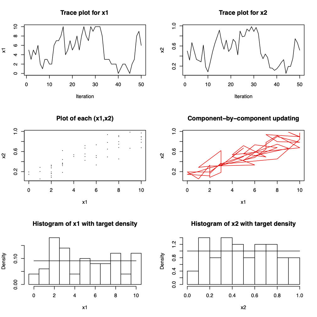
Figure 3.7: Fifty iterations from a Gibbs sampler for \(x_{1} | x_{2} \sim Bin(n, x_{2})\), \(x_{2} | x_{1} \sim Beta(x_{1} + \alpha, n - x_{1} + \beta)\) where \(n=10\) and \(\alpha = \beta = 1\). The marginal distributions are \(x_{1} \sim Beta-binomial(n, \alpha, \beta)\) and \(x_{2} \sim Beta(\alpha, \beta)\). For \(\alpha = \beta = 1\), \(x_{1}\) is the discrete uniform on \(\{0,1, \ldots, n\}\) and \(x_{2} \sim U(0, 1)\).

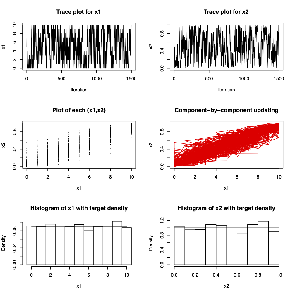
Figure 3.8: 1500 iterations from a Gibbs sampler for \(x_{1} | x_{2} \sim Bin(n, x_{2})\), \(x_{2} | x_{1} \sim Beta(x_{1} + \alpha, n - x_{1} + \beta)\) where \(n=10\) and \(\alpha = \beta = 1\). The marginal distributions are \(x_{1} \sim Beta-binomial(n, \alpha, \beta)\) and \(x_{2} \sim Beta(\alpha, \beta)\). For \(\alpha = \beta = 1\), \(x_{1}\) is the discrete uniform on \(\{0,1, \ldots, n\}\) and \(x_{2} \sim U(0, 1)\).

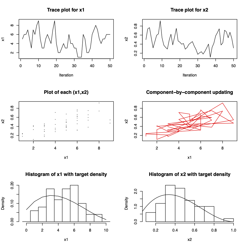
Figure 3.9: Fifty iterations from a Gibbs sampler for \(x_{1} | x_{2} \sim Bin(n, x_{2})\), \(x_{2} | x_{1} \sim Beta(x_{1} + \alpha, n - x_{1} + \beta)\) where \(n=10\), \(\alpha = 2\) and \(\beta = 3\). The marginal distributions are \(x_{1} \sim Beta-binomial(n, \alpha, \beta)\) and \(x_{2} \sim Beta(\alpha, \beta)\).

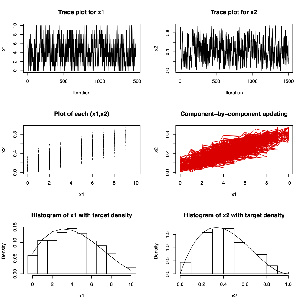
Figure 3.10: 1500 iterations from a Gibbs sampler for \(x_{1} | x_{2} \sim Bin(n, x_{2})\), \(x_{2} | x_{1} \sim Beta(x_{1} + \alpha, n - x_{1} + \beta)\) where \(n=10\), \(\alpha = 2\) and \(\beta = 3\). The marginal distributions are \(x_{1} \sim Beta-binomial(n, \alpha, \beta)\) and \(x_{2} \sim Beta(\alpha, \beta)\).

Notice that the Gibbs sampler for \(\theta = (\theta_{1}, \ldots, \theta_{d})\) can be viewed as a special case of the Metropolis-Hastings algorithm where each iteration \(t\) consists of \(d\) Metropolis-Hastings steps each with an acceptance probability of 1. We shall show this in question 4 of Question Sheet Eight.

3.3.4 A brief insight into why the Metropolis-Hastings algorithm works

A topic of major importance when studying Markov chains is determining the conditions under which there exists a stationary distribution and what that stationary distribution is. In MCMC methods, the reverse approach is taken. We have a stationary distribution \(\pi\) (typically a posterior distribution from which we wish to sample) and we want to find the transition probabilities of a Markov chain which has \(\pi\) as the stationary distribution.

In this section we shall motivate why the Metropolis-Hastings works. For ease of understanding we shall work in the discrete setting. The case when the state space of the Markov chain is continuous follows very similarly, largely by the usual approach of replacing sums by integrals.

Consider a discrete Markov chain \(X_{t}\) with transition probabilities, see (3.6), \[\begin{eqnarray} P_{\theta \phi} & = & P(X_{t} = \phi \, | \, X_{t-1} = \theta) \nonumber \end{eqnarray}\] for all \(\theta\), \(\phi \in S\), the state space of the chain. To make the link between the discrete and continuous case more explicit we shall let \[\begin{eqnarray} P_{\theta \phi} = q_{1}(\phi \, | \, \theta). \nonumber \end{eqnarray}\] Suppose that the chain has a stationary distribution, for example from Theorem 3.1 a sufficient condition is that the chain is irreducible and aperiodic, \(\pi\).

From Definition 3.5, think of \(\pi_{i} = \pi(\theta)\), \(\pi_{j} = \pi(\phi)\) and \(P_{ij} = P_{\theta \phi} = q_{1}(\phi \, | \, \theta)\), the stationary distribution \(\pi = \{\pi(\theta) : \theta \in S\}\) satisfies \[\begin{eqnarray} \pi(\phi) & = & \sum_{\theta \in S} \pi(\theta)q_{1}(\phi \, | \, \theta). \tag{3.10} \end{eqnarray}\] In the continuous case we have \[\begin{eqnarray} \pi(\phi) & = & \int_{\theta} \pi(\theta)q_{1}(\phi \, | \, \theta) \, d\theta \nonumber \end{eqnarray}\] highlighting the replacement of sums by integrals.

Notice that, as the chain must move somewhere, \[\begin{eqnarray} \sum_{\phi \in S} q_{1}(\phi \, | \, \theta) & = & 1. \tag{3.11} \end{eqnarray}\] If the equation \[\begin{eqnarray} \pi(\theta)q_{1}(\phi \, | \, \theta) & = & \pi(\phi)q_{1}(\theta \, | \, \phi) \tag{3.12} \end{eqnarray}\] is satisfied for all \(\theta\), \(\phi\) then the \(q_{1}(\phi \, | \, \theta)\) satisfy time reversibility or detailed balance. If (3.12) holds then the \(q_{1}(\phi \, | \, \theta)\) are the transition probabilities of a Markov chain with stationary distribution \(\pi\) since \[\begin{eqnarray} \sum_{\theta \in S} \pi(\theta)q_{1}(\phi \, | \, \theta) & = & \sum_{\theta \in S} \pi(\phi)q_{1}(\theta \, | \, \phi) \tag{3.13} \\ & = & \pi(\phi) \sum_{\theta \in S} q_{1}(\theta \, | \, \phi)\nonumber\\ & = & \pi(\phi) \tag{3.14} \end{eqnarray}\] which is (3.10), where (3.13) follows from (3.12) and (3.14) from (3.11).

We now demonstrate how, by considering detailed balance, we can derive the Metropolis-Hastings algorithm. Let \(q(\phi \, | \, \theta)\) denote the proposal density of a scheme where we wish to sample from \(\pi(\theta)\). Typically, \(q(\cdot)\) will be easy to sample from and the sufficient conditions for the existence of a stationary distribution (aperiodicity and irreducibility), \(\pi(\theta)\), are mopped up in \(q(\cdot)\). In a Bayesian context, we will usually wish to sample from the posterior so that \(\pi(\theta) = f(\theta \, | \, x)\). We propose a move from \(\theta\) to \(\phi\) with probability \[\begin{eqnarray} \alpha(\theta, \phi) & = & \min \left(1, \frac{\pi(\phi)q(\theta \, | \, \phi)}{\pi(\theta)q(\phi \, | \, \theta)}\right). \nonumber \end{eqnarray}\] The transition probabilities of the Markov chain created using the Metropolis-Hastings algorithm are \[\begin{eqnarray} q_{1}(\phi \, | \, \theta) & = & \left\{\begin{array}{ll} q(\phi \, | \, \theta)\alpha(\theta, \phi) & \phi \neq \theta \\ 1 - \sum_{\phi \neq \theta} q(\phi \, | \, \theta)\alpha(\theta, \phi) & \phi = \theta.\end{array}\right. \nonumber \end{eqnarray}\] (There are two ways for \(q_{1}(\theta \, | \, \theta)\): either we reject a proposed move to \(\phi \neq \theta\) or we sample \(\theta = \phi\).) We now show that \(q_{1}(\phi \, | \, \theta)\) satisfies detailed balance. For \(\phi \neq \theta\) we have \[\begin{eqnarray} \pi(\theta)q_{1}(\phi \, | \, \theta) & = & \pi(\theta)q(\phi \, | \, \theta)\alpha(\theta, \phi) \nonumber \\ & = & \pi(\theta)q(\phi \, | \, \theta) \min \left(1, \frac{\pi(\phi)q(\theta \, | \, \phi)}{\pi(\theta)q(\phi \, | \, \theta)}\right) \nonumber \\ & = & \min\left(\pi(\theta)q(\phi \, | \, \theta), \pi(\phi)q(\theta \, | \, \phi)\right) \nonumber \\ & = & \pi(\phi)q(\theta \, | \, \phi) \min \left(1, \frac{\pi(\theta)q(\phi \, | \, \theta)}{\pi(\phi)q(\theta \, | \, \phi)}\right) \nonumber \\ & = & \pi(\phi)q(\theta \, | \, \phi)\alpha(\phi, \theta) \nonumber \\ & = & \pi(\phi)q_{1}(\theta \, | \, \phi). \nonumber \end{eqnarray}\] Thus, using (3.12), \(\pi(\theta)\) is the stationary distribution of the Markov chain created using the Metropolis-Hastings algorithm with proposal distribution \(q(\phi \, | \, \theta)\).

3.3.5 Efficiency of the algorithms

The efficiency of the Metropolis-Hastings algorithm depends upon a “good” choice of proposal density \(q(\phi \, | \, \theta)\). In practice we want

1. A high acceptance probability: we don’t want to repeatedly sample points we reject. Practical experience suggests that a “good” \(q(\phi \, | \, \theta)\) will be close to \(f(\theta \, | \, x)\) but slightly heavier in the tails.

2. To explore the whole distribution: we want a good coverage of all possible values of \(\theta\) and not to spend too long in only a small area of the distribution.

A chain that does not move around very quickly is said to be slow mixing.

The Gibbs sampler accepts all new points so we don’t need to worry about the acceptance probability. However, we may experience slow mixing if the parameters are highly correlated. Ideally we want the parameters to be as close to independence as possible as sampling from conditionals reduces to sampling directly from the desired marginals.

Example 3.7 Suppose that we want to use a Gibbs sampler to sampler from the posterior \(f(\theta \, | \, x)\) where \(\theta = (\theta_{1}, \ldots, \theta_{d})\). For the Gibbs sampler we sample from the conditionals \(f(\theta_{i} \, | \, \theta_{-i}, x)\) for \(i = 1, \ldots, d\) where \(\theta_{-i} = \theta \setminus \theta_{i}\). If the \(\theta_{i}\) are independent then \[\begin{eqnarray} f(\theta \, | \, x) & = & \prod_{i=1}^{d} f(\theta_{i} \, | \, x) \nonumber \end{eqnarray}\] and \(f(\theta_{i} \, | \, \theta_{-i}, x) = f(\theta_{i} \, | \, x)\). The Gibbs sampler will sample from the posterior marginal densities.

In some cases, it may be worthwhile to deal with reparameterisations of \(\theta\), for example using a reparameterisation which makes the parameters close to independent.

3.3.6 Using the sample for inference

The early values of a chain, before convergence, are called the . The length of burn-in will depend upon the rate of convergence of the Markov chain and how close to the posterior we need to be. In general, it is difficult to obtain estimates of the rate of convergence and so analytically determining the length of burn-in required is not feasible. A practitioner uses times series plots of the chain as a way of judging convergence. Suppose that we judge convergence to have been reached after \(b\) iterations of an MCMC algorithm have been performed. We discard the observations \(\theta^{(1)}, \ldots, \theta^{(b)}\) and work with the observations \(\{\theta^{(t)} : t > b\}\) which are viewed as being a sample from the stationary distribution of the Markov chain which is typically the posterior distribution.