Chapter 1 The Bayesian method

We shall adopt the notation \(f(\cdot)\) (some authors use \(p(\cdot)\)) to represent the density function, irrespective of whether the random variable over which the distribution is specified is continuous or discrete. In general notation we shall make no distinction as to whether random variables are univariate or multivariate. In specific examples, if necessary, we shall make the dimension explicit.

1.1 Bayes’ theorem

Let \(X\) and \(Y\) be random variables with joint density function \(f(x, y)\). The marginal distribution of \(Y\), \(f(y)\), is the joint density function averaged over all possible values of \(X\), \[\begin{eqnarray} f(y) & = & \int_{X} f(x, y) \, dx. \tag{1.1} \end{eqnarray}\] For example, if \(Y\) is univariate and \(X = (X_{1}, X_{2})\) where \(X_{1}\) and \(X_{2}\) are univariate then \[\begin{eqnarray} f(y) & = & \int_{-\infty}^{\infty}\int_{-\infty}^{\infty} f(x_{1}, x_{2}, y) \, dx_{1} dx_{2}. \nonumber \end{eqnarray}\] The conditional distribution of \(Y\) given \(X = x\) is \[\begin{eqnarray} f(y \, | \, x) & = & \frac{f(x, y)}{f(x)} \tag{1.2} \end{eqnarray}\] so that by substituting (1.2) into (1.1) we have \[\begin{eqnarray} f(y) & = & \int_{X} f(y \, | \, x)f(x)\, dx. \nonumber \end{eqnarray}\] which is often known as the theory of total probability. \(X\) and \(Y\) are independent if and only if \[\begin{eqnarray} f(x, y) & = & f(x)f(y). \tag{1.3} \end{eqnarray}\] Substituting (1.2) into (1.3) we see that an equivalent result is that \[\begin{eqnarray} f(y \, | \, x) & = & f(y) \nonumber \end{eqnarray}\] so that independence reflects the notion that learning the outcome of \(X\) gives us no information about the distribution of \(Y\) (and vice versa). If \(Z\) is a third random variable then \(X\) and \(Y\) are conditionally independent given \(Z\) if and only if \[\begin{eqnarray} f(x, y \, | \, z) & = & f(x \, | \, z)f(y \, | \, z). \tag{1.4} \end{eqnarray}\] Note that \[\begin{eqnarray} f(y \, | \, x, z) & = & \frac{f(x, y, z)}{f(x, z)} \nonumber \\ & = & \frac{f(x, y \, | \, z)f(z)}{f(x \, | \, z)f(z)} \nonumber \\ & = & \frac{f(x, y \, | \, z)}{f(x \, | \, z)} \tag{1.5} \end{eqnarray}\] so, by substituting (1.4) into (1.5), an equivalent result to (1.4) is that \[\begin{eqnarray} f(y \, | \, x, z) & = & f(y \, | \, z). \nonumber \end{eqnarray}\] Thus, conditional independence reflects the notion that having observed \(Z\) then there is no further information about \(Y\) that can be gained by additionally observing \(X\) (and vice versa for \(X\) and \(Y\)).

Theorem 1.1 (Bayes' theorem) For \(f(x) > 0\), \[\begin{eqnarray} f(y \, | \, x) & = & \frac{f(x \, | \, y)f(y)}{f(x)} \tag{1.6} \\ & = & \frac{f(x \, | \, y)f(y)}{\int_{Y} f(x \, | \, y)f(y) \, dy}. \nonumber \end{eqnarray}\]

Bayes’ theorem is named after Thomas Bayes (c1701-1761).

1.2 Bayes’ theorem for parameteric inference

Consider a general problem in which we have data \(x\) and require inference about a parameter \(\theta\). In a Bayesian analysis \(\theta\) is unknown and viewed as a random variable. Thus, it possesses a density function \(f(\theta)\).

Note that Bayes’ theorem holds for any random variables. In a Bayesian analysis, \(\theta\) is a random variable and so Bayes’ theorem can be utilised for probability distributions concerning \(\theta\).

From Bayes’ theorem, (1.6), we have \[\begin{eqnarray} f(\theta \, | \, x) & = & \frac{f(x \, | \, \theta)f(\theta)}{f(x)} \nonumber \\ & \propto & f(x \, | \, \theta)f(\theta). \tag{1.7} \end{eqnarray}\] Colloquially (1.7) is \[\begin{eqnarray} \mbox{Posterior} & \propto & \mbox{Likelihood} \times \mbox{Prior}. \nonumber \end{eqnarray}\] Most commonly, both the parameter \(\theta\) and data \(x\) are continuous. There are cases, such as the Bernoulli trials case in Example 0.1, when \(\theta\) is continuous and \(x\) is discrete. In exceptional cases \(\theta\) could be discrete.

The Bayesian method comprises of the following principle steps.

1. Prior
   Obtain the prior density \(f(\theta)\) which expresses our knowledge about \(\theta\) prior to observing the data.

2. Likelihood
   Obtain the likelihood function \(f(x \, | \, \theta)\). This step simply describes the process giving rise to the data \(x\) in terms of \(\theta\).

3. Posterior
   Apply Bayes’ theorem to derive posterior density \(f(\theta \, | \, x)\) which expresses all that is known about \(\theta\) after observing the data.

4. Inference
   Derive appropriate inference statements from the posterior distribution e.g. point estimates, interval estimates, probabilities of specified hypotheses.

1.3 Sequential data updates

It is important to note that the Bayesian method can be used sequentially. Suppose we have two sources of data \(x\) and \(y\). Then our posterior for \(\theta\) is \[\begin{eqnarray} f(\theta \, | \, x, y) & \propto & f(x, y \, | \, \theta)f(\theta). \tag{1.8} \end{eqnarray}\] Now \[\begin{eqnarray} f(x, y \, | \, \theta)f(\theta) \ = \ f(x, y, \theta) & = & f(y \, | \, x, \theta)f(x, \theta) \nonumber \\ & = & f(y \, | \, x, \theta)f(\theta \, | \, x)f(x) \nonumber \\ & \propto & f(y \, | \, x, \theta)f(\theta \, | \, x) \tag{1.9} \end{eqnarray}\] Substituting (1.9) into (1.8) we have \[\begin{eqnarray} f(\theta \, | \, x, y) & \propto & f(y \, | \, x, \theta)f(\theta \, | \, x). \tag{1.10} \end{eqnarray}\] We can update first by \(x\) and then by \(y\). Note that, in this case, \(f(\theta \, | \, x)\) assumes the role of the prior (given \(x\)) and \(f(y \, | \, x, \theta)\) the likelihood (given \(x\)).

1.4 Conjugate Bayesian updates

Example 1.1 Beta-Binomial. Suppose that \(X \, | \, \theta \sim Bin(n, \theta)\). We specify a prior distribution for \(\theta\) and consider \(\theta \sim Beta(\alpha, \beta)\) for \(\alpha, \beta > 0\) known. Thus, for \(0 \leq \theta \leq 1\) we have \[\begin{eqnarray} f(\theta) & = & \frac{1}{B(\alpha, \beta)} \theta^{\alpha - 1}(1 - \theta)^{\beta -1} \tag{1.11} \end{eqnarray}\] where \(B(\alpha, \beta) = \frac{\Gamma(\alpha)\Gamma(\beta)}{\Gamma(\alpha + \beta)}\) is the beta function and \(E(\theta) = \frac{\alpha}{\alpha + \beta}\). Recall that as \[\begin{eqnarray} \int_{0}^{1} f(\theta) \, d\theta & = & 1 \nonumber \end{eqnarray}\] then \[\begin{eqnarray} B(\alpha, \beta) & = & \int_{0}^{1} \theta^{\alpha - 1}(1 - \theta)^{\beta -1} \, d\theta. \tag{1.12} \end{eqnarray}\]

Using Bayes’ theorem, (1.7), the posterior is \[\begin{eqnarray} f(\theta \, | \, x) \ \propto \ f(x \, | \, \theta)f(\theta) & = & \binom{n}{x}\theta^{x}(1-\theta)^{n-x} \times \frac{1}{B(\alpha, \beta)} \theta^{\alpha - 1}(1 - \theta)^{\beta -1} \nonumber \\ & \propto & \theta^{x}(1-\theta)^{n-x}\theta^{\alpha - 1}(1 - \theta)^{\beta -1}\nonumber\\ & = & \theta^{\alpha + x - 1}(1 - \theta)^{\beta + n - x -1}. \tag{1.13} \end{eqnarray}\] So, \(f(\theta \, | \, x) = c\theta^{\alpha + x - 1}(1 - \theta)^{\beta + n - x -1}\) for some constant \(c\) not involving \(\theta\). Now \[\begin{eqnarray} \int_{0}^{1} f(\theta \, | \, x) \, d\theta \ = \ 1 & \Rightarrow & c^{-1} \ = \ \int_{0}^{1} \theta^{\alpha + x - 1}(1 - \theta)^{\beta + n - x -1} \, d\theta. \nonumber \end{eqnarray}\] Notice that from (1.12) we can evaluate this integral so that \[\begin{eqnarray} c^{-1} \ = \ \int_{0}^{1} \theta^{\alpha + x - 1}(1 - \theta)^{\beta + n - x -1} \, d\theta \ = \ B(\alpha + x, \beta + n - x) \nonumber \end{eqnarray}\] whence \[\begin{eqnarray} f(\theta \, | \, x) & = & \frac{1}{B(\alpha + x, \beta + n - x)} \theta^{\alpha + x - 1}(1 - \theta)^{\beta + n - x -1} \nonumber \end{eqnarray}\] i.e. \(\theta \, | \, x \sim Beta(\alpha + x, \beta + n - x)\).

Notice the tractability of this update: the prior and posterior distribution are both from the same family of distributions, in this case the Beta family. This is an example of conjugacy. The update is simple to perform: the number of successes observed, \(x\), is added to \(\alpha\) whilst the number of failures observed, \(n - x\), is added to \(\beta\).

We treated \(\alpha, \beta > 0\) as known. It is possible to consider \(\alpha\) and/or \(\beta\) to be random variables and then specify prior distributions for them. This would be an example of a hierarchical Bayesian model.

Definition 1.1 (Conjugate family) A class \(\Pi\) of prior distributions is said to form a conjugate family with respect to a likelihood \(f(x \, | \, \theta)\) if the posterior density is in the class of \(\Pi\) for all \(x\) whenever the prior density is in \(\Pi\).

In Example 1.1 we showed that, with respect to the Binomial likelihood, the Beta distribution is a conjugate family.

One major advantage of Example 1.1, and conjugacy in general, was that it was straightforward to calculate the constant of proportionality. In a Bayesian analysis we have \(f(\theta \, | \, x) \propto f(x \, | \, \theta)f(\theta)\) so that \(f(\theta \, | \, x) = cf(x \, | \, \theta)f(\theta)\) where \(c\) is a constant not involving \(\theta\). As \(f(\theta \, | \, x)\) is a density function and thus integrates to unity we have \[\begin{eqnarray} c^{-1} & = & \int_{\theta} f(x \, | \, \theta)f(\theta) \, d\theta. \nonumber \end{eqnarray}\] In practice, it is not always straightforward to compute this integral and no closed form for it may exist.

We will now explore the effect of the prior and the likelihood on the posterior. To ease the comparison we will view the likelihood as a function of \(\theta\) and consider the standardised likelihood \(\frac{f(x \, | \, \theta)}{\int_{\theta} f(x \, | \, \theta) \, d\theta}\), that is scaled so that the area under the curve is unity. Note that this is only appropriate when the integral on the denominator is finite - there are instances when this is not the case.

We shall use the Beta distribution as an example. The Beta distribution is an extremely flexible distribution on \((0, 1)\) and, as Figure 1.1 shows, careful choice of the parameters \(\alpha\), \(\beta\) can be used to create a wide variety of shapes for the prior density.

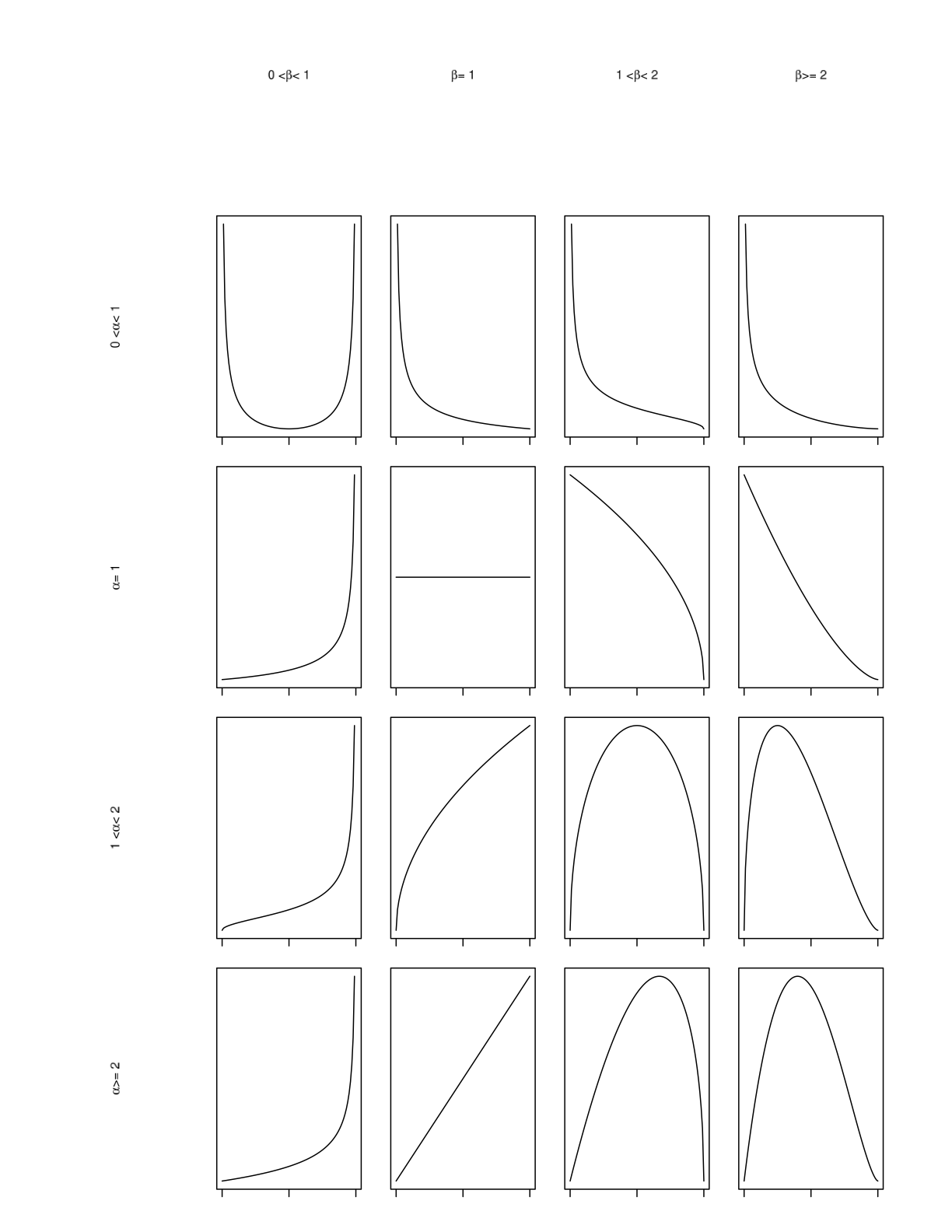
Figure 1.1: A plot of the Beta distribution, \(Beta(\alpha, \beta)\), for varying choices of the parameters \(\alpha\), \(\beta\)

Example 1.2 Recall Example 0.3. We consider the two experiments.

1. Toss a coin \(n\) times and observe \(x\) heads. Parameter \(\theta_{c}\) represents the probability of tossing a head on a single trial.

2. Toss a drawing pin \(n\) times and observe that the pin lands facing upwards on \(x\) occasions.

In both cases we have a Binomial likelihood and I judge that a Beta distribution can be used to model my prior beliefs about both \(\theta_{c}\) and \(\theta_{p}\). I have considerably more prior knowledge about \(\theta_{c}\) than \(\theta_{p}\). In particular, I am confident that \(E(\theta_{c}) = \frac{1}{2}\) and that the distribution is pretty concentrated around this point, so that the variance is small. If I model my beliefs about \(\theta_{c}\) with a Beta distribution then \(E(\theta_{c}) = \frac{1}{2}\) implies that I must take \(\alpha = \beta\). I judge that the \(Beta(20, 20)\) distribution adequately models my prior knowledge about \(\theta_{c}\). I have considerably less knowledge about \(\theta_{p}\) but I have no reason to think the process is unfair so take \(E(\theta_{p}) = \frac{1}{2}\). However, I reflect my lack of knowledge about \(\theta_{p}\), compared certainly to \(\theta_{c}\), with a large variance so that the distribution is less concentrated around the mean. I judge that the \(Beta(2, 2)\) distribution adequately models my prior knowledge about \(\theta_{p}\).

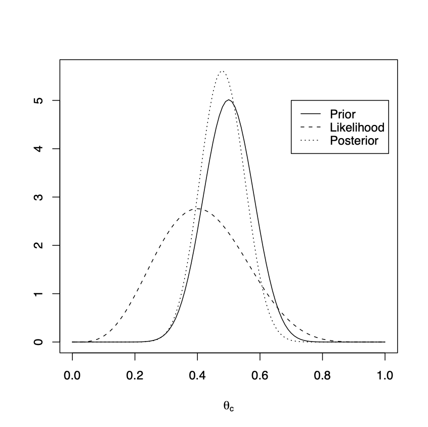
Suppose that, in each case, I perform \(n = 10\) tosses and observe \(x = 4\) successes. We may use Example 1.1 to compute the posterior for \(\theta_{c}\) and for \(\theta_{p}\). \[\begin{eqnarray} & \begin{array}{c|ccc} & \mbox{Prior} & \mbox{Likelihood} & \mbox{Posterior} \\ \hline \theta_{c} & Beta(20, 20) & x=4, n=10 & Beta(24, 26) \\ \theta_{p} & Beta(2, 2) & x=4, n=10 & Beta(6, 8) \\ \end{array} \nonumber \end{eqnarray}\] We plot the prior density, standardised likelihood and posterior density for both \(\theta_{c}\) and \(\theta_{p}\).

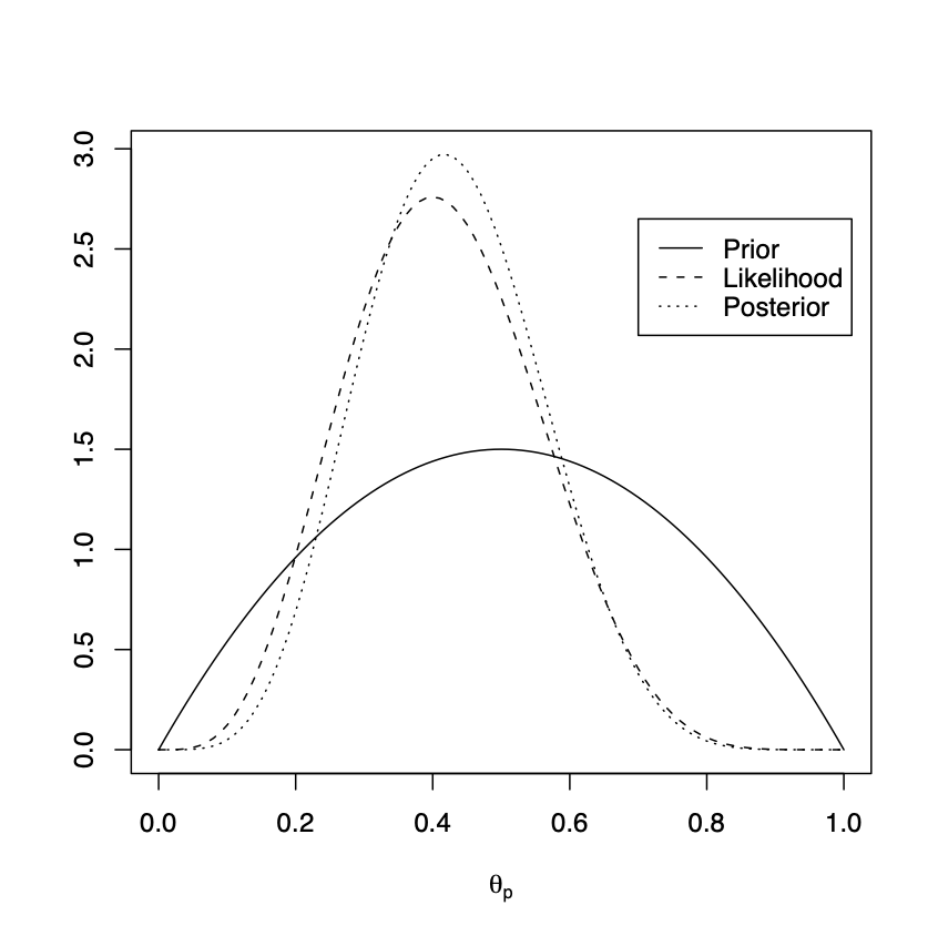
Figure 1.2: Left, tossing coins. Prior \(\theta_{c} \sim Beta(20, 20)\), posterior \(\theta_{c}|x \sim Beta(24, 26)\). Right, tossing drawing pins. Prior \(\theta_{p} \sim Beta(2, 2)\), posterior \(\theta_{p}|x \sim Beta(6, 8)\).

In Figure 1.2 we plot the prior density, standardised likelihood and posterior density for both \(\theta_{c}\) and \(\theta_{p}\). Notice how, for \(\theta_{c}\), the strong prior information is reflected by the posterior density closely following the prior density. The mode of the posterior is shifted to the left of the prior, towards the mode of the likelihood, reflecting that the maximum likelihood estimate (\(\frac{4}{10}\)) was smaller than the prior suggested. The posterior density is (slightly) taller and narrower than the prior reflecting the new information about \(\theta_{c}\) from the data. For \(\theta_{p}\), the weaker prior information can be seen by the fact that the posterior density now much more follows the (standardised) likelihood - most of our posterior knowledge about \(\theta_{p}\) is coming from the data. Notice how the posterior density is much taller and narrower than the prior reflecting how the data resolves a lot of the initial uncertainty about \(\theta_{p}\).

Notice that in our calculation of \(f(\theta \, | \, x)\), see (1.13), we were only interested in quantities proportional to \(f(\theta \, | \, x)\) and we identified that \(\theta \, | \, x\) was a Beta distribution by recognising the form \(\theta^{\tilde{\alpha}-1}(1-\theta)^{\tilde{\beta}-1}\).

Definition 1.2 (Kernal of a density) For a random variable \(X\) with density function \(f(x)\) if \(f(x)\) can be expressed in the form \(cq(x)\) where \(c\) is a constant, not depending upon \(x\), then any such \(q(x)\) is a kernel of the density \(f(x)\).

Example 1.3 If \(\theta \sim Beta(\alpha, \beta)\) then \(\theta^{\alpha-1}(1-\theta)^{\beta-1}\) is a kernel of the \(Beta(\alpha, \beta)\) distribution.

Spotting kernels of distributions can be very useful in computing posterior distributions.

Example 1.4 In Example 1.1 we can find the posterior distribution \(\theta \, | \, x\) by observing that (1.13) is a kernel of the \(Beta(\alpha + x, \beta + n - x)\) distribution.

Example 1.5 Let \(X\) be normally distribution with unknown mean \(\theta\) and known variance \(\sigma^{2}\). It is judged that \(\theta \sim N(\mu_{0}, \sigma_{0}^{2})\) where \(\mu_{0}\) and \(\sigma_{0}^{2}\) are known.

For the prior we have \[\begin{eqnarray} f(\theta) & = & \frac{1}{\sqrt{2\pi} \sigma_{0}} \exp \left\{-\frac{1}{2\sigma_{0}^{2}}(\theta - \mu_{0})^{2}\right\} \nonumber \\ & \propto & \exp \left\{-\frac{1}{2\sigma_{0}^{2}}(\theta - \mu_{0})^{2}\right\} \tag{1.14} \\ & \propto & \exp \left\{-\frac{1}{2\sigma_{0}^{2}}(\theta^{2} - 2\mu_{0}\theta)\right\} \tag{1.15} \end{eqnarray}\] where (1.14) and (1.15) are both kernels of the normal distribution. For the likelihood we have \[\begin{eqnarray} f(x \, | \, \theta) & = & \frac{1}{\sqrt{2\pi} \sigma} \exp \left\{-\frac{1}{2\sigma^{2}}(x - \theta)^{2}\right\} \nonumber \\ & \propto & \exp \left\{-\frac{1}{2\sigma^{2}}(\theta^{2} - 2 x \theta)\right\} \tag{1.16} \end{eqnarray}\] where, since \(f(x \, | \, \theta)\) represents the likelihood, in (1.16) we are only interested in \(\theta\). For the posterior, from (1.15) and (1.16), we have \[\begin{eqnarray} f(\theta \, | \, x) & \propto & \exp \left\{-\frac{1}{2\sigma^{2}}(\theta^{2} - 2 x \theta)\right\}\exp \left\{-\frac{1}{2\sigma_{0}^{2}}(\theta^{2} - 2\mu_{0}\theta)\right\} \nonumber \\ & = & \exp\left\{-\frac{1}{2}\left(\frac{1}{\sigma^{2}} + \frac{1}{\sigma_{0}^{2}}\right)\left[\theta^{2} - 2\left(\frac{1}{\sigma^{2}} + \frac{1}{\sigma_{0}^{2}}\right)^{-1}\left(\frac{x}{\sigma^{2}}+\frac{\mu_{0}}{\sigma_{0}^{2}}\right)\theta\right]\right\} \tag{1.17} \end{eqnarray}\] We recognise (1.17) as a kernel of a normal distribution so that \(\theta \, | \, x \sim N(\mu_{1}, \sigma_{1}^{2})\) where \[\begin{eqnarray} \sigma_{1}^{2} & = & \left(\frac{1}{\sigma^{2}} + \frac{1}{\sigma_{0}^{2}}\right)^{-1} \tag{1.18} \\ \mu_{1} & = & \left(\frac{1}{\sigma^{2}} + \frac{1}{\sigma_{0}^{2}}\right)^{-1}\left(\frac{x}{\sigma^{2}}+\frac{\mu_{0}}{\sigma_{0}^{2}}\right) \tag{1.19} \end{eqnarray}\] Notice that we can write (1.18) as \[\begin{eqnarray} \frac{1}{\sigma_{1}^{2}} & = & \frac{1}{\sigma^{2}} + \frac{1}{\sigma_{0}^{2}} \nonumber \end{eqnarray}\] so that the posterior precision is the sum of the data precision and the prior precision.

Recall that the precision is the reciprocal of the variance. The lower the variance the higher the precision.

From (1.19) we observe that the posterior mean is a weighted average of the data and the prior mean, weighted according to the corresponding precisions. The posterior mean will be closest to whichever of the prior and likelihood has the stronger information. For example, if the prior information is very weak, expressed by large \(\sigma_{0}^{2}\) and thus small precision, then \(\mu_{1}\) will be close to the data \(x\).

We note that with respect to a normal likelihood (with known variance), the normal distribution is a conjugate family.

1.5 Using the posterior for inference

Our posterior beliefs are captured by a whole distribution \(f(\theta \, | \, x)\). Typically we want to summarise this distribution. We might use

1. Graphs and plots of the shape of the distribution.

2. Measures of location such as the mean, median and mode.

3. Measures of dispersion such as the variance, quantiles e.g. quartiles, interquartile range.

4. A region that captures most of the values of \(\theta\).

5. Other relevant summaries e.g. the posterior probability that \(\theta\) is greater than some value.

We shall focus upon the fourth of these points. In the discussion that follows we shall assume that \(\theta\) is univariate: the results and definitions simply generalise for the case when \(\theta\) is multivariate.

1.5.1 Credible intervals and highest density regions

Credible intervals (or posterior intervals) are the Bayesian analogue of confidence intervals. A \(100(1-\alpha)\%\) confidence interval for a parameter \(\theta\) is interpreted as meaning that with a large number of repeated samples \(100(1-\alpha)\%\) of the corresponding confidence intervals would contain the true value of \(\theta\).

Repeated sampling is a cornerstone of classical statistics. There are a number of issues with this e.g. the long-run repetitions are hypothetical, what do we do when we can only make a finite number of realisations or an event occurs once and once only.

A \(100(1-\alpha)\%\) credible interval is an actual interval that contains the parameter \(\theta\) with probability \(1 - \alpha\).

Definition 1.3 (Credible interval) A \(100(1-\alpha)\%\) credible interval \((\theta_{L}, \theta_{U})\) is an interval within which \(100(1-\alpha)\%\) of the posterior distribution lies, \[\begin{eqnarray} P(\theta_{L} < \theta < \theta_{U} \, | \, x) \ = \ \int_{\theta_{L}}^{\theta_{U}} f(\theta \, | \, x) \, d\theta \ = \ 1 - \alpha. \nonumber \end{eqnarray}\]

The generalisation for multivariate \(\theta\) is a region \(C\) contained within the probability space of \(\theta\) which contains \(\theta\) with probability \(1 - \alpha\).

Notice that there are infinitely many such intervals. Typically we fix the interval by specifying the probability in each tail. For example, we frequently take \[\begin{eqnarray} P(\theta < \theta_{L} \, | \, x) \ = \ \frac{\alpha}{2} \ = \ P(\theta > \theta_{U} \, | \, x). \nonumber \end{eqnarray}\] We can explicitly state that there is a \(100(1-\alpha)\%\) probability that \(\theta\) is between \(\theta_{L}\) and \(\theta_{U}\). Observe that we can construct similar intervals for any (univariate) random variable, in particular for the prior. In such a case the interval is often termed a prior credible interval.

Example 1.6 Recall Example 1.2. We construct 95% prior credible intervals and credible intervals for the two cases of tossing coins and drawing pins. We elect to place 2.5% in each tail. The intervals may be found using R and the command qbeta(0.025, a, b) for \(\theta_{L}\) and for \(\theta_{U}\) qbeta(0.975, a, b). \[\begin{eqnarray} & \begin{array}{c|cccc} & \mbox{Prior} & \mbox{Prior credible} & \mbox{Posterior} & \mbox{(Posterior) credible} \\ \hline \theta_{c} & Beta(20, 20) & (0.3478, 0.6522) & Beta(24, 26) & (0.3442, 0.6173) \\ \theta_{p} & Beta(2, 2) & (0.0950, 0.9057) & Beta(6, 8) & (0.1922, 0.6842) \\ \end{array} \nonumber \end{eqnarray}\] Notice that the prior credible interval and (posterior) credible interval for \(\theta_{c}\) cover a similar location: this is not a surprise as, from the left hand plot of Figure 1.2, we observed that the prior and posterior distributions for \(\theta_{c}\) were very similar with the latter shifted slightly to the left in the direction of the likelihood. This feature is reflected in the interval \((0.3442, 0.6173)\) covering the left hand side of \((0.3478, 0.6522)\). The width of the credible interval is also narrower: 0.2731 compared to 0.3044 for the prior credible interval. This is an illustration of the data reducing our uncertainty about \(\theta_{c}\).

Note that, see the solution to Question Sheet One 5(b), for generic parameter \(\theta\) and data \(x\) we have \(Var(\theta) = Var(E(\theta \, | \, X)) + E(Var(\theta \, | \, X))\) so that \(E(Var(\theta \, | \, X)) \leq Var(\theta)\): we expect the observation of data \(x\) to reduce our uncertainty about parameter \(\theta\).

For \(\theta_{p}\) the prior credible interval has a width of 0.8107 reflecting the weak prior knowledge. Observation of the data shrinks the width of this interval considerably to 0.4920 which is still quite wide (wider than the initial prior credible interval for \(\theta_{c}\)) which is not surprising: we had only weak prior information and the posterior, see the right hand plot of Figure 1.2, closely mirrors the likelihood. We observed only ten tosses so we would not anticipate that the data would resolve most, or indeed much, of the uncertainty about \(\theta_{p}\).

Definition 1.4 (Highest density region) The highest density region (HDR) is a region \(C\) that contains \(100(1-\alpha)\%\) of the posterior distribution and has the property that for all \(\theta_{1} \in C\) and \(\theta_{2} \notin C\), \[\begin{eqnarray} f(\theta_{1} \, | \, x) & \geq & f(\theta_{2} \, | \, x). \nonumber \end{eqnarray}\]

Thus, for a HDR the density insider the region is never lower than outside of the region. The HDR is the region with \(100(1-\alpha)\%\) probability of containing \(\theta\) with the shortest total length. For unimodal symmetric distributions the HDR and credible interval are the same. Credible intervals are generally easier to compute (particularly if we are doing so by placing \(\frac{\alpha}{2}\) in each tail) and are invariant to transformations of the parameters. HDRs are more complex and there is a potential lack of invariance under parameter transformation. However, they may be more meaningful for multinomial distributions.

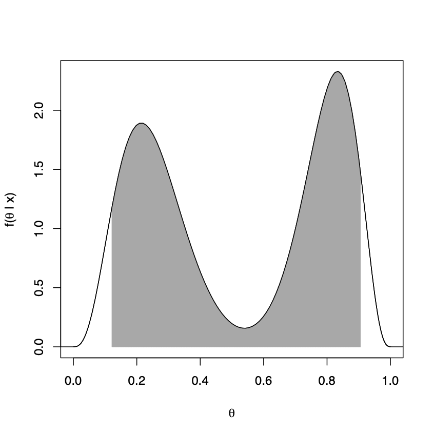
Example 1.7 Figure 1.3 shows a 90% credible interval and HDR for a parameter \(\theta\) whose posterior distribution, given by \(f(\theta \, | \, x)\), is bimodal.

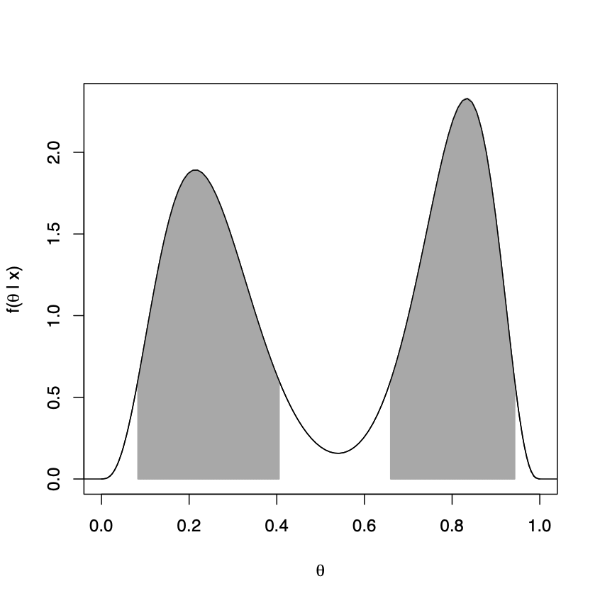
Figure 1.3: Left, shaded area denotes 90% credible interval for a bimodal distribution with 5% in each tail. Right, shaded areas denote 90% highest density region for the bimodal distribution.

The plotted density is a mixture of a \(Beta(4, 12)\) and a \(Beta(16, 4)\) with \(f(\theta \, | \, x) = \frac{1}{2B(4, 12)}\theta^{3}(1-\theta)^{11} + \frac{1}{2B(16, 4)}\theta^{15}(1-\theta)^{3}\).

Notice that the credible interval, see the left hand plot of Figure 1.3, is not a HDR. In particular, \(\theta_{1} = 0.5\) is in the credible interval and \(\theta_{2} = 0.95\) is not and \(f(0.95 \, | \, x) > f(0.5 \, | \, x)\). Moreover, the credible interval may not be sensible. For example, it includes the interval \((0.5, 0.6)\) which has a small probability of containing \(\theta\). The HDR is shown in the right hand plot of Figure 1.3. It consists of two disjoint intervals and thus captures the bimodality of the distribution. It has a total length of 0.61 compared to the total length of 0.78 for the credible interval.