Chapter 5 Numerical linear algebra

Problem For a given \(d\times d\) matrix \(A\) and vector \(\vec b \in \mathbb{R}^d\), find \(\vec x\in\mathbb{R}^d\) such that \(A\vec x=\vec b\). If the entries of \(A\) are \(a_{ij}\) (row \(i\), column \(j\)) and the entries of \(\vec x\) and \(\vec b\) are \(x_j\) and \(b_j\), this means \[ \sum_{j=1}^d a_{ij} x_j =b_i,\qquad i=1,\cdots,d. \]

You have studied already row-reduction techniques. In numerical analysis, these are developed in a way to improve numerical stability into the standard technique “Gaussian elimination with partial pivoting”. This is an example of a direct method and this means the solution \(\mathbf x\) is found by a finite number of arithmetic operations. Packages such as scipy.linalg use Gaussian elimination to find an LU factorisation.

Definition 5.1 A matrix \(P\) is a permutation matrix if each row and column has exactly one non-zero entry equal to one; multiplication by a permutation matrix \(P\) in \(PA\) permutes the rows of \(A\).

A matrix \(L\) is lower triangular if \(L_{ij}=0\) for \(i< j\) and unit lower triangular if additionally \(L_{ii}=1\). A matrix \(U\) is upper triangular if \(U_{ij}=0\) for \(i> j\).

The LU factorisation consists of a permutation matrix \(P\), a unit lower-triangular matrix \(L\), and an upper-triangular matrix \(U\) such that \(PA=LU\); this can be found in Python using P, L, U = scipy.linalg.lu(A). For example,

\[ L= \begin{bmatrix} 1 & 0 & 0 \\ 0 & 1 & 0 \\ 1/2 & 1/2 & 1 \end{bmatrix},\quad% U= \begin{bmatrix} 4 & -1 & 1 \\ 0 & -1 & 2\\ 0 & 0 & -3/2 \end{bmatrix},\quad% P=\begin{bmatrix} 0 & 1 & 0 \\ 0 & 0 & 1\\ 1 & 0 & 0 \end{bmatrix} \] is an LU factorisation of \[ A= \begin{bmatrix} 2 & -1 & 0\\ 4 & -1 & 1\\ 0 & -1 & 2 \end{bmatrix}. \]

You should verify that \(PA=LU\). The entries of \(L\) and \(U\) express the row reductions normally performed in Gaussian elimination. We do not show how to compute \(L\) and \(U\) in detail by hand. There are many matrix factorisation in numerical linear algebra and this one is useful for solving linear systems of equations.

Example 5.1 (LU factorisation) To solve a linear system of equations with the LU factorisation, substitute \(PA=LU\) into the linear system \(A\vec x=\vec b\): \[ PA \vec x=L U \vec x= P \vec b. \] Let \(\vec y:= U \vec x\). Given \(\vec b\in\mathbb{R}^d\), we solve the triangular system \[ L \vec y=P \vec b, \qquad \text{to find $\,\vec y\in\mathbb{R}^d$} \] and \[ U \vec x= \vec y,\qquad \text{to find $\,\vec x\in \mathbb{R}^d$.} \] We have replaced the problem of solve \(A\vec x=\vec b\) by solving two much simpler linear systems. Both matrices are triangular and their solution is easily found by forward or backward substitution.

We spend most of our time studying iterative methods, where \(\vec x\) occurs as the limit of approximations \(\vec x_n\) as \(n\to \infty\). In general, direct methods (such as the LU factorisation or Gaussian elimination) are good for dense matrices (where \(a_{ij}\ne 0\) for nearly all \(i,j\)) and the complexity of such a linear solve is \(\mathcal{O}(d^3)\). If \(d\) is very large, it may be impossible to store \(A\) in memory and to perform row reductions. On the other hand, the matrix may be sparse (\(a_{ij}=0\) for many \(i,j\)) and it may be easy to compute matrix-vector products \(A \vec x\). In this case, iterative methods are valuable.

We will work with the following example of a sparse matrix throughout.

Example 5.2 (finite-difference matrix) Suppose that \(u\) is a smooth real-valued function on \([0,1]\) and we want to approximate its second derivative based on evaluations on the mesh \(x_i=ih\) for some mesh spacing \(h=1/(d+1)\). By Taylor’s theorem, \[\begin{align*} u(x+h)&=u(x)+h u'(x)% +\frac 12 h^2 u''(x)% +\frac 16 h^3 u'''(x)+\mathcal{O}(h^4),\\ u(x-h)&=u(x)-h u'(x)% +\frac 12 h^2 u''(x)% -\frac 16 h^3 u'''(x)+\mathcal{O}(h^4). \end{align*}\]

Then, \[ u''(x)% =\frac{u(x+h)-2u(x)+u(x-h)}{h^2}% +\mathcal{O}(h^2). \] By dropping the \(\mathcal{O}(h^2)\) term, we have a finite-difference approximation to the second derivative. This can be used to find an approximate solution to the two-point boundary value problem: for a given function \(f:[0,1]\to\mathbb{R}\), find \(u(x)\) such that \[ -u''(x)=f(x),\qquad u(0)=u(1)=0. \] Using the finite-difference approximation, \[ -\begin{bmatrix} u''(x_1)\\ u''(x_2)\\\vdots\\u''(x_d) \end{bmatrix} =\frac{1}{h^2} A \begin{bmatrix} u(x_1)\\ u(x_2)\\\vdots\\u(x_d) \end{bmatrix}+\mathcal{O}(h^2) \] for \[\begin{equation} \tag{5.1} A:= \begin{bmatrix} 2 & -1 & & \\ -1& 2 & -1 & \\ & \ddots & \ddots& \ddots \\ & &-1& 2 \end{bmatrix}. \end{equation}\] Then \(u''(x)=-f(x)\) gives \(\frac{1}{h^2}A \vec u= f\) if we neglect the \(\mathcal{O}(h^2)\) term, for \[\begin{equation} f:=\begin{bmatrix} f(x_1)\\ f(x_2)\\\vdots\\f(x_d) \end{bmatrix},\quad \vec u:=\begin{bmatrix} u(x_1)\\ u(x_2)\\\vdots\\u(x_d) \end{bmatrix}. \end{equation}\] We have a linear system of equations that can be solved to determine an approximate solution of the boundary-value problem.

Only the main and two off-diagonals of \(A\) are non-zero. All other entries are zero and the matrix is sparse. We will use the finite-difference matrix \(A\) as a prototype example as we develop iterative methods. The matrix is typical of the ones that arise in the numerical solution of PDEs.

5.1 Iterative methods

Suppose we wish to solve \(A\vec x=\vec b\) for \(\vec x\in\mathbb{R}^d\) given a \(d\times d\) matrix \(A\) and \(\vec b\in\mathbb{R}^d\). Write \(A=A_1-A_2\) so that \[ A_1\vec x= A_2 \vec x+ \vec b. \] This motivates the following iterative method: find \(\vec x_{n+1}\) such that \[ A_1 \vec x_{n+1}% =A_2 \vec x_n+\vec b. \] When \(\vec x_n\) is known and \(A_1\) is well chosen, we easily find \(\vec x_{n+1}\) and generate a sequence \(\vec x_1,\vec x_2,\dots\) that we hope converges to the solution \(\vec x\). We can interpret this as a fixed-point iteration and \[ \vec x_{n+1}=\vec g(\vec x_n),\qquad \vec g(\vec x):= A_1^{-1}(A_2\vec x+\vec b), \] where we assume the inverse matrix \(A_1^{-1}\) exists.

Example 5.3 (Jacobi) Let \(A_1\) denote the diagonal part of \(A\) and \(A_2=A_1-A=-(L+U)\) (for the lower- and upper-triangular parts \(L\) and \(U\) of \(A\)). Take for example \[ A= \begin{bmatrix} 2&-1\\-1&2 \end{bmatrix},\qquad A_1= \begin{bmatrix} 2&0\\0&2 \end{bmatrix},\qquad A_2= \begin{bmatrix} 0&1\\1&0 \end{bmatrix}. \] The Jacobi iteration is \[ \begin{bmatrix} 2 & 0 \\ 0 &2 \end{bmatrix}\vec x_{n+1}% = \begin{bmatrix} 0 &1\\1 & 0 \end{bmatrix}\vec x_n +\vec b \] or \[ \vec x_{n+1} = \begin{bmatrix} 0 & 1/2 \\ 1/2 & 0 \end{bmatrix}\vec x_n + \frac 12 \vec b. \] Notice how simple it is to evaluate the right-hand side given \(\vec x_n\) and \(\vec b\).

For the finite-difference example (5.1), the Jacobi method is \[\begin{equation} \tag{5.2} \vec x_{n+1}=\frac 12 \begin{bmatrix} 0&1 & & & \\ 1&\ddots &1 & & \\ & \ddots& &\ddots & \\ &&&&1\\ &&& 1& \end{bmatrix}\vec x_n% +\frac12 \vec b. \end{equation}\] Even when \(d\) is large, the right-hand side is cheap to compute and the matrix-vector product is easy to evaluate without storing the sparse matrix.

Example 5.4 (Gauss-Seidel) Let \(A_1=D+L\) (the diagonal and lower-triangular part) and \(A_2=-U\). For the finite-difference matrix, \[ \underbrace{ \begin{bmatrix} 2 & & & \\ -1& 2 & & \\ &-1& 2 & \\ &&\ddots&\ddots & \\ \end{bmatrix}}_{=A_1}\vec x_{n+1}% =\underbrace{\begin{bmatrix} 0& 1 & & & \\ &\ddots &1 & \\ && &1 \\ &&&\ddots & \\ \end{bmatrix}}_{=A_2}\vec x_{k}+\vec b% \] This time a linear solve is required. As the matrix on the left-hand side is lower triangular, this can be done efficiently to find \(\vec x_{n+1}\).

We now develop some tools for understanding the convergence of iterative methods.

5.2 Vector and matrix norms

To understand convergence of \(\vec x_n\), we introduce a way to measure distance on \(\mathbb{R}^d\). It turns out to be very convenient to have more than one measurement of distance.

Definition 5.2 (vector norm) A vector norm on \(\mathbb{R}^d\) is a real-valued function \(\|\cdot\|\) on \(\mathbb{R}^d\) such that

1. \(\|\vec x\|\ge 0\) for all \(\vec x\in \mathbb{R}^d\),
2. \(\|\vec x\|=0\) if and only if \(\vec x=\vec 0\),
3. \(\|\alpha \vec x\|=|\alpha|\,\|\vec x\|\) for \(\alpha\in \mathbb{R}\), and
4. \(\|\vec x+\vec y\|\le \|\vec x\|+\|\vec y\|\) for all \(\vec x, \vec y\in\mathbb{R}^d\) (the triangle inequality).

The standard Euclidean norm \(\|\vec x\|_2:= \big(\vec x^\mathsf{T} \vec x\big)^{1/2}\equiv \big(x_1^2+\dots+x_d^2\big)^{1/2}\) satisfies these conditions and is a vector norm. The conditions (a–c) are easy to verify. The last one follows from the Cauchy-Schwarz inequality, which says that \(\vec x^\mathsf{T} \vec y \le \|\vec x\|_2 \|\vec y\|_2\) and so \[\begin{align*} \|\vec x+\vec y\|_2^2% &= (\vec x+\vec y)^\mathsf{T} (\vec x+\vec y)\\ & =\vec x^\mathsf{T} \vec x + 2 \vec x^\mathsf{T} \vec y+ \vec y^\mathsf{T} \vec x\\[2pt] & \le \|\vec x\|_2^2 + 2 \|\vec x\|_2 \|\vec y\|_2 + \|\vec y\|_2^2\\ & = \big(\|\vec x\|_2 + \|\vec y|_2\big)^2. \end{align*}\] We will make use of two more examples: \[ \|\vec x\|_\infty% := \max_{j=1,\dots, d}|x_j|,\qquad \|\vec x\|_1% := \sum_{j=1}^{d}|x_j|. \]

Don’t forget the absolute-value signs on the right-hand side! Verification of the norm axioms is straightforward here.

These give different numbers and, for \(\vec x=(-1,1,2)^\mathsf{T}\), we get \[ \|\vec x\|_2=\sqrt{6},\qquad \|\vec x\|_1=4,\qquad \|\vec x\|_\infty=2. \]

We also need to measure matrices. The obvious way to do this is to treat a \(d\times d\) matrix as a \(d^2\) vector and thereby inherit the norms defined for vectors. This does not say anything about the multiplicative nature of matrices and so we develop the following concept.

Definition 5.3 (matrix norm) A matrix norm \(\|A\|\) of a \(d\times d\) matrix \(A\) is a real-valued function on \(\mathbb{R}^{d\times d}\) such that

1. \(\|A\| \ge 0\) for all \(A\in \mathbb{R}^{d\times d}\),
2. \(\|A\| = 0\) if and only if \(A=0\),
3. \(\|\alpha A\| = |\alpha|\,\|A\|\) for \(\alpha\in \mathbb{R}\),
4. \(\|A+B\| \le \|A\| + \|B\|\) (the triangle inequality) and
5. \(\|A B\| \le \|A\|\,\|B\|\) for all \(A, B\in\mathbb{R}^{d\times d}\).

Conditions (a–d) correspond to the ones for vector norms. The last, the sub-multiplicative condition, relates to matrix products.

Vector norms lead naturally to a corresponding matrix norm, known as the subordinate or operator norm.

Definition 5.4 The operator norm \(\|A\|_{\mathrm{op}}\) with respect to a vector norm \(\|\vec x\|\) is defined by \[ \|A\|_{\mathrm{op}} := \sup_{\vec x\ne 0} \frac{\|A\vec x\|}{\|\vec x\|}. \] Equivalently, because of condition (c), \[ \|A\|_{\mathrm{op}} = \sup_{\|\vec x\|=1}{\|A\vec x\|} \] (\(\sup\) means least upper bound or roughly “the maximum”. However, since the hypersphere \(\{\vec x : \|\vec x\|=1\}\) is compact, the supremum in this case can be replaced by a maximum.).

The operator norm describes the maximum stretch that can be achieved by multiplication by \(A\).

Theorem 5.1 The operator norm \(\|A\|_{\mathrm{op}}\) is a matrix norm

Proof. We show (e). As \(\|A\|_{\mathrm{op}}=\sup \|A\vec x\|/\|\vec x\|\), we have \[\begin{equation} \tag{5.3} \|A \vec x\|% \le \|A\|_{\mathrm{op}} \|\vec x\| \end{equation}\] for any \(\vec x\in \mathbb{R}^d\). Then, applying (5.3) twice, \[ \|A B \vec x\|% \le \|A\|_{\mathrm{op}} \|B\vec x\|% \le \|A\|_{\mathrm{op}} \|B\|_{\mathrm{op}} \|\vec x\|. \] Hence, \[ \|AB\|_{\mathrm{op}}% =\sup_{\|\vec x\|=1} \|A B \vec x\| \le \|A\|_{\mathrm{op}} \|B\|_{\mathrm{op}}. \] The remaining conditions are left for a problem sheet.

Let \(\|A\|_1\) be the operator norm associated to the vector norm \(\|\vec x\|_1\), and \(\|A\|_\infty\) be the operator norm associated to the vector norm \(\|\vec x\|_\infty\).

Theorem 5.2 Let \(A\) be an \(d\times d\) matrix. Then, \[\begin{align*} \|A\|_1&% =\max_{j=1,\dots,d} \sum_{i=1}^d |a_{ij}|,\qquad \text{maximum column sum}\\ \|A\|_\infty&% =\max_{i=1,\dots,d} \sum_{j=1}^d |a_{ij}|,\qquad \text{maximum row sum}. \end{align*}\]

To remember which way round it is, \(\|A\|_1\) is the maximum column sum and the subscript \(1\) looks like a column. Don’t forget the absolute-value signs!

Proof. We prove that \[ \|A\|_\infty=\max_i \sum_j|a_{ij}| =: f(A). \] The argument for \(\|A\|_1\) is similar and addressed on the problem sheet. We divide and conquer, first showing that \(\|A\|_\infty \le f(A)\) and then \(\|A\|_\infty \ge f(A).\)

To show that \(\|A\|_\infty \le f(A)\), consider \(\vec x\in\mathbb{R}^d\) with \(\|\vec x\|_\infty=1\). Then, \(|x_i|\le 1\) for all \(i=1,\dots,d\) and hence \[ \bigg|\sum_{j=1}^d a_{ij}\, x_j\bigg|% \le\sum_{j=1}^d |a_{ij}\, x_j|% \le \sum_{j=1}^d |a_{ij}|% \le f(A). \] That is, the \(i\)th entry of \(A\vec x\) is smaller (in absolute value) than \(f(A)\). Hence, \(\|A\vec x\|_\infty \le f(A)\).

To show that \(\|A\|_\infty \ge f(A)\), suppose that \(f(A)=\sum_j |a_{ij}|\) (i.e., row \(i\) has the maximum sum). Let \[ x_j% := \begin{cases} +1,& a_{ij}\ge 0,\\ -1, & a_{ij}<0. \end{cases} \] Clearly then \(\|\vec x\|_\infty=1\) and \[ A\vec x = \begin{bmatrix} \times\\\times\\\vdots\\ \sum_j a_{ij} x_j\\ \times \end{bmatrix}% = \begin{bmatrix} \times\\\times\\\vdots \\ \sum_j |a_{ij}| \\\times \end{bmatrix}= \begin{bmatrix} \times\\ \times\\\vdots \\ f(A) \\ \times \end{bmatrix}, \] where we write the \(i\)th row only. The magnitude of the largest entry of \(A\vec x\) is at least \(f(A)\) and \[ \|A\vec x\|_\infty \ge f(A), \] completing the proof.

Both these operator norms are very easy to compute.

Example 5.5 Let \[ A= \begin{bmatrix} 3 &-8& -9\\ 1 &-2& 0\\ 9 &-14& 6 \end{bmatrix}. \] Then \(\|A\|_1=\max\{13, 24,15\}=24\) and \(\|A\|_\infty=\max\{20,3,29\}=29\).

The matrix 2-norm \(\|A\|_2\) induced by the Euclidean vector norm \(\|\vec x\|_2\) is much harder to understand. We quote the following theorem:

Theorem 5.3 Let \(A\) be a \(d\times d\) matrix; then \[\begin{equation} \tag{5.4} \|A\|_2% =\sqrt{\rho(A^\mathsf{T} A)}, \end{equation}\] where \(\rho(B)\) is the spectral radius or size of the largest eigenvalue defined by \[\rho(B):= \max\{|\lambda| : \text{$\lambda$ is an eigenvalue of $B$ so that $B\vec u=\lambda \vec u$ for some $\vec u\ne \vec 0$}\}.\] When \(A\) is symmetric, we have simply that \[ \|A\|_2= \rho(A). \]

The proof of (5.4) is not covered. In the symmetric case, \(A=A^\mathsf{T}\) and, if \(\lambda\) is an eigenvalue of \(A\), then \(\lambda^2\) is an eigenvalue of \(A^\mathsf{T} A=A^2\). We expect \(\rho(A^\mathsf{T} A)=\rho(A)^2\).

Eigenvalues of large matrices are difficult to compute, though we can easily do it for a \(2\times 2\) example.

Example 5.6 Let \[ A= \begin{bmatrix} 3 & 1 \\ 0 &1 \end{bmatrix}, \qquad A^\mathsf{T} A= \begin{bmatrix} 9 & 3 \\ 3 &2 \end{bmatrix}. \] The eigenvalues \(\lambda\) are the solutions of \[ \det(A-\lambda I)% =\det{ \begin{vmatrix} 9-\lambda & 3 \\ 3 & 2-\lambda \end{vmatrix}}% =(9-\lambda)(2-\lambda) -9 =\lambda^2-11\lambda+9=0. \] The quadratic equation formula gives \(\lambda=(11\pm \sqrt{121-36})/2\) and \(\|A\|_2=\rho(A)=\sqrt{(11+\sqrt{85})/2}\).

Example 5.7 Recall the \(d\times d\) finite-difference matrix \[ A% = \begin{bmatrix} 2& -1 & & \\ -1 & 2 &-1 & \\ & \ddots&\ddots&\ddots \\ \\ \end{bmatrix}. \] We find the eigenvalues of \(A\), which allows us to find \(\|A\|_2\). Let \(h:= 1/(d+1)\) and \[ \vec u_k% := ( \sin k\pi h, \sin 2k\pi h, \dots, \sin d k \pi h)^\mathsf{T}% \in \mathbb{R}^d. \] We show that \(\vec u_k\) is an eigenvector of \(A\). The \(j\)th component of \(A\vec u_k\) is \[ (A \vec u_k)_j% = 2 \sin (j k \pi h)% - \sin((j-1) k \pi h)% - \sin((j+1)k \pi h), \] where we use \(\sin((j-1)k\pi h)=0\) for \(j=1\) and \(\sin((j+1)k \pi h)=\sin(k \pi)=0\) for \(j=d\).

The trig identity \(\sin(X+Y)=\cos X \sin Y+\cos Y \sin X\) gives \[\begin{align*} (A \vec u_k)_j% &= 2 \sin (j k \pi h) - (\cos (k\pi h) \sin (j k \pi h) - \cos (j k \pi h) \sin (k \pi h))\\ &\qquad- (\cos (k \pi h) \sin (j k \pi h) + \cos (j k \pi h) \sin( k \pi h))\\[2pt] &= 2(1-\cos k \pi h) \sin (j k \pi h)\\[2pt] &= \lambda_k \times \text{the $j$th component of $\vec u_k$,} \end{align*}\] where \(\lambda_k:= 2(1-\cos (k\pi h))\). In other words, \(\lambda_k\) is an eigenvalue of \(A\) with eigenvector \(\vec u_k\). This gives \(d\) distinct eigenvalues for \(A\). We conclude that \[ \rho(A)% = \max \{ \lambda_k: k=1,\dots,d \}% =2\bigg(1-\cos \frac{d\pi}{d+1}\bigg). \] As \(A\) is symmetric, Theorem 5.3 gives \[ \|A\|_2% =\sqrt{\rho(A^\mathsf{T} A)}% =\rho(A)% =2\bigg(1-\cos \frac{d\pi}{d+1}\bigg). \]

5.3 Convergence of iterative methods

If \(A=D+L+U\) (sum of diagonal and lower- and upper-triangular parts), the Jacobi method is \[ D \vec x_{n+1}=-(L+U) \vec x_n+\vec b \] and the Gauss-Seidel method is \[ (L+D) \vec x_{n+1} = -U \vec x_n + \vec b. \] If \(D\) is non-singular, both can be written \[ \vec x_{n+1}% =T \vec x_n+\vec c \] where \[\begin{alignat*}{3} T=T_{\textrm J} &:= -D^{-1}(L+U),& \qquad \vec c &=D^{-1} \vec b, &\qquad &\text{Jacobi},\\ T=T_{\textrm GS} &:= -(L+D)^{-1}U,& \qquad \vec c&=(L+D)^{-1} \vec b, &\qquad &\text{Gauss-Seidel}. \end{alignat*}\]

Lemma 5.1 Suppose that \(A\) and \(D\) are non-singular. Consider \(T=T_{\mathrm J}\) or \(T=T_{\mathrm{GS}}\). Then \(\vec x\) is the solution of \(A\vec x=\vec b\) if and only if \(\vec x=\vec g(\vec x):= T\vec x+\vec c\) (i.e., \(\vec{x}\) is a fixed point of \(\vec g\); see Definition 4.1).

Proof. Elementary.

Theorem 5.4 Suppose that the conditions of Lemma 5.1 hold, so that \(A \vec x=\vec b\) has a unique solution \(\vec x\). Suppose that \(\vec x_n\) is a sequence in \(\mathbb{R}^d\) generated by \[\begin{equation*} \vec x_{n+1} = T \vec x_n+\vec c, \end{equation*}\] for some initial vector \(\vec x_0\). Then, \[ \|\vec x_n-\vec x\|% \le \|T\|_{\mathrm{op}}^n \|\vec x_0-\vec x\|, \] where \(\|T\|_{\mathrm{op}}\) is the operator norm associated to a vector norm \(\|\vec x\|\).

Proof. We have \(\vec x_{n+1}=T\vec x+\vec c\) and \(\vec x=T \vec x+\vec c\); then \[ \vec x_{n+1}-\vec x% = (T\vec x_n-T \vec x)% + (\vec c-\vec c). \] Apply the vector norm: \[ \|\vec x_{n+1}-\vec x\|% =\|T\vec x_n-T \vec x\|. \] Using (5.3), \[ \|\vec x_{n+1}-\vec x\|% \le\|T\|_{\mathrm{op}}\,\|\vec x_n- \vec x\|. \] As simple induction argument shows that \(\|\vec x_{n}-\vec x\| \le \|T\|_{\mathrm{op}}^n \|\vec x_0-\vec x\|.\)

Corollary 5.1 If \(\|T\|_{\mathrm{op}}<1\), then \(\vec x_n\) converges to \(\vec x\) as \(n\to \infty\). The convergence is linear (see Definition 4.2); that is, \(\|\vec x_{n+1}-\vec x\|\le K \|\vec x_n-\vec x\|\) for \(K=\|T\|_{\mathrm{op}}<1\).

When \(\|T\|_{\mathrm{op}}\) is small, the convergence is more rapid and this is desirable in numerical calculations.

In finite dimensions, it turns out that all norms are equivalent and any operator norm can be used as long as \(\|T\|_{\mathrm{op}}<1\).

An alternative characterisation of convergence can be given in terms of eigenvalues.

Corollary 5.2 The sequence \(\vec x_{n}\) given by \(\vec x_{n+1}=T\vec x_n+\vec c\) converges to the fixed point \(\vec x\) satisfying \(\vec x=T\vec x+\vec c\) for any \(\vec x_0\in \mathbb{R}^d\) if \(\rho(T)<1\).

Proof. This is a corollary of Theorem 5.4 when \(T\) is symmetric as \(\rho(T)=\|T\|_2\).

Suppose for simplicity that \(T\) has \(d\) distinct eigenvalues \(\lambda_j\) with corresponding eigenvectors \(\vec u_j\), so that \(T \vec u_j=\lambda_j \vec u_j\). Then, \(\vec u_j\) is a basis for \(\mathbb{R}^d\) and \[ \vec x_0-\vec x=\sum_{j=1}^d \alpha_j \vec u_j, \] for some \(\alpha_j\in\mathbb{R}\). Let \(\vec e_n=\vec x_n-\vec x\). Then, \(\vec e_{n+1}=T\vec e_n\) and \[ \vec e_{n}% =T^n \vec e_0% =T^n \sum_{j=1}^d \alpha_j \vec u_j% = \sum_{j=1}^d\alpha_j T^n \vec u_j% = \sum_{j=1}^d \alpha_j \lambda^n \vec u_j. \] If \(\rho(T)<1\) then all eigenvalues \(\lambda\) satisfy \(|\lambda|<1\). Hence, \(\lambda^n \to 0\) as \(n\to \infty\). Thus \(\vec e_n\to 0\) as \(n\to \infty\) and the iterative method converges.

The case where the eigenvalues of \(T\) are not distinct is omitted.

Example 5.8 Consider \[ \begin{bmatrix} 8 & -1 & 0 \\ 1 & 5 & 2 \\ 0 & 2 & 4 \end{bmatrix}% \vec x% = \vec b% = \begin{bmatrix} 1 \\2 \\3 \end{bmatrix}. \] The Jacobi iteration is \[ \begin{bmatrix} 8 &0 &0 \\ 0& 5 &0 \\0 &0 &4 \end{bmatrix} \vec x_{n+1}% = \begin{bmatrix} 0 & 1 & 0\\ -1 & 0 &-2 \\ 0& -2 & 0 \end{bmatrix}\vec x_n + \begin{bmatrix} 1 \\ 2 \\3 \end{bmatrix} \] and \[ T_J = \begin{bmatrix} 8 & 0&0 \\0 & 5 &0 \\0 &0 &4 \end{bmatrix}^{-1} \begin{bmatrix} 0 & 1 & 0\\ -1 & 0 &-2 \\ 0& -2 & 0 \end{bmatrix}% = \begin{bmatrix} 0 & 1/8 & 0\\ -1/5 & 0 & -2/5\\ 0 & -1/2 & 0 \end{bmatrix}. \] Then, \[ \|T_J\|_\infty= \max\left\{\frac 18, \frac 35, \frac 12\right\}% =\frac 35,\qquad \text{max row sum} \] \[ \|T_J\|_1 = \max\left\{\frac 15, \frac 58, \frac 25\right\}% =\frac 58,\qquad \text{max column sum}. \] The matrix norms are less than one and the Jacobi iteration converges for this example.

Example 5.9 (finite-difference matrix) Recall the Jacobi iteration for the finite-difference matrix (5.2). Then, \(\vec x_{n+1}=T \vec x_n+\vec c\) for \[ T% = \frac 12 \begin{bmatrix} 0&1 & & & \\ 1&\ddots &1 & & \\ & \ddots& &\ddots & \\ &&&&&1\\ &&&& 1& 0 \end{bmatrix}, \qquad% \vec c% =\frac 12 \vec b. \]

Note that \(\|T\|_\infty=\|T\|_1=1\) so that Corollary 5.1 does not apply. We work out the eigenvalues similarly to Example 5.7. Let \(\vec u_k=[\sin( k\pi h),\sin (2k\pi h),\dots, \sin (d k \pi h)]^\mathsf{T}\) for \(h=1/(d+1)\). Then, the \(j\)th component of \(T\vec u_k\) is \(\frac 12 (\sin(j-1)k \pi h) + \sin (j+1) k\pi h)\) and, by applying a trig identity, this is \(\cos (k\pi h) \sin(j k \pi h)\). Thus, \(\lambda_k=\cos (k\pi h)\) for \(k=1,\dots,d\) are the eigenvalues of \(T\) and, as \(|\lambda_k|<1\), the convergence of the Jacobi iteration follows for the finite-difference matrix.

Note however that \(\rho(T)=\max\{\cos (k\pi h): k=1,\dots,d\}\to 1\) as \(h\to 0\) as \(\cos (\pi h)\approx 1\) for \(h\approx 0\). This means when \(h\) is small the Jacobi iteration converges slowly. This is a significant problem in applications where small \(h\) corresponds to accurate resolution of the underlying physics. In other words, the more accurate our discretisation the slower the Jacobi iteration is.

For convergence of Gauss-Seidel with the finite-difference matrix, see Problem Sheets.

5.4 Condition number

We’d like to estimate the error in the approximation when solving a linear system. Our methods provide a computed value \(\vec x_c\) that we hope approximates the solution \(\vec x\) of \(A\vec x=\vec b\). We cannot evaluate a norm for \(\vec x_c-\vec x\) as \(\vec x\) is usually unknown. What we do have is the residual defined by \[ \vec r:= A\vec x_c-\vec b. \] Note that \[ \vec r:= A\vec x_c-A\vec x= A(\vec x_c-\vec x) \] and \(\vec x_c-\vec x=A^{-1} \vec r\). Apply (5.3) to get \[ \|\vec x_c-\vec x\|\le \|A^{-1}\|_{\mathrm{op}} \|\vec r\|. \] Furthermore, \(A\vec x=\vec b\) gives \[ \|\vec b\|=\|A\vec x\| \le \|A\|_{\mathrm{op}}\, \|\vec x\|. \] Dividing the two expressions, \[ \frac{\|\vec x_c-\vec x\|}{\|A\|_{\mathrm{op}}\,\|\vec x\|}% \le \frac{\|A^{-1}\|_{\mathrm{op}} \, \|\vec r\|}{\|\vec b\|}. \] Rearranging we get \[ \underbrace{\frac{\|\vec x_c-\vec x\|}{\|\vec x\|}}_{\text{relative error}}% \le \underbrace{\vphantom{\frac{\\|x\|}{\|x\|}}\|A^{-1}\|_{\mathrm{op}}\, \|A\|_{\mathrm{op}}}_{\text{condition number}} \, \underbrace{\frac{\|\vec r\|}{\|\vec b\|}.}_{\text{relative residual}} \] Thus, the relative error is bounded by a constant times the relative residual. The constant is known as the condition number:

Definition 5.5 (condition number) The condition number of a non-singular matrix \(A\) is defined by \[ \mathrm{Cond}(A)% :=\|A\|_{\mathrm{op}}\,\|A^{-1}\|_{\mathrm{op}}. \] Each choice of operator norm \(\|A\|_{\mathrm{op}}\) gives a different condition corresponding to the choice of vector norm \(\|\vec x\|\) above and \(\mathrm{Cond}_1(A)\), \(\mathrm{Cond}_2(A)\), \(\mathrm{Cond}_\infty(A)\) denote the condition numbers with respect to the \(1\)-, \(2\)-, and \(\infty\)-norms. Often \(\kappa(A)\) is used to denote the condition number.

The condition number is a widely used measure of the difficulty of solving \(A\vec x=\vec b\). When \(\mathrm{Cond}(A)\) is large, it may be impossible to get accurate results.

Example 5.10 Returning to (1.1), we have \[ A= \begin{bmatrix} \epsilon & 1 \\ 0 & 1 \end{bmatrix},\qquad A^{-1}= \frac 1 \epsilon\begin{bmatrix} 1 & -1 \\ 0 & \epsilon \end{bmatrix}. \] Suppose that \(0<\epsilon<1\). Then, \(\|A\|_1=2\) and \(\|A^{-1}\|_1=(1+\epsilon)/\epsilon\) and hence \(\mathrm{Cond}_1(A)=2(1+\epsilon)/\epsilon\). This is large when \(\epsilon\) is small and the matrix is ill-conditioned. This reflects the sensitivity of \(\vec x\) to changes in \(\vec b\) found when solving \(A\vec x=\vec b\) in (1.1).

Example 5.11 (Hilbert matrix) Refer back to Problem Sheet 1 where we performed experiments with the Hilbert matrix \(A\), which is the \(d\times d\) matrix with \((i,j)\) entry \(1/(i+j-1)\). We found that it was difficult to solve the linear system of equations \(A\vec x=\vec b\) for a given \(\vec b\in\mathbb{R}^d\) if \(d\) is moderately large (e.g., \(d=10\)). In Python, numpy.linalg provides the command cond for finding the condition number. We apply this to the Hilbert matrix

  from numpy.linalg import cond
  from scipy.linalg import hilbert
  d = 4
  A = hilbert(d)
  cond_A = cond(A,p=1)
  print(A, cond_A)

The output is

  [[1.         0.5        0.33333333 0.25      ]
   [0.5        0.33333333 0.25       0.2       ]
   [0.33333333 0.25       0.2        0.16666667]
   [0.25       0.2        0.16666667 0.14285714]]
  28374.99999999729

Repeating this experiment for \(d=6\) we find a condition number of \(2.9070\times 10^7\); for \(d=8\), the condition number is \(3.3872\times 10^{10}\); for \(d=10\), the condition number is \(3.534\times 10^{13}\). Even for small systems (problem in real-world applications can be easily have millions of unknowns), the condition number is extremely large.

5.4.1 Second derivation of \(\operatorname{cond}(A)\)

Suppose that \[ A\vec x= \vec b,\qquad (A+\Delta A)\vec x_c= \vec b,\qquad \] where \(\Delta A\) can be thought as the effects of rounding error. Then, \[ \vec x=A^{-1} \vec b= A^{-1}(A+\Delta A) \vec x_c% =\vec x_c+ A^{-1} \Delta A \vec x_c\,. \] Hence, \[ \vec x-\vec x_c = A^{-1} \Delta A \vec x_c\,. \] Applying norms, we find that \[ \|\vec x-\vec x_c\| \le \|A^{-1}\|_{\mathrm{op}} \|\Delta A\|_{\mathrm{op}} \| \vec x_c\|. \] We can rewrite this in terms of the condition number: \[ \frac{\|\vec x-\vec x_c\|}{\|\vec x_c\|} \le \mathrm{Cond}(A) \frac{\|\Delta A\|_{\mathrm{op}}}{\|A\|_{\mathrm{op}}}. \] The relative error is less than the condition number times the size of the relative change in \(A\).

Example 5.12 (finite-difference matrix) Let \(A\) be the \(d\times d\) finite-difference matrix of Example 5.2. Then, \(\mathrm{Cond}_2(A)\) is easy to find, because we know all the eigenvalues of \(A\). The eigenvalues of \(A^{-1}\) are simply \(\lambda^{-1}\) where \(\lambda\) is an eigenvalue of \(A\). So, as \(A\) is symmetric, \[ \mathrm{Cond}_2(A)=\|A\|_2 \|A^{-1}\|_2=\rho(A) \rho(A^{-1}). \] The eigenvalues are \(\lambda_k=2(1-\cos (k\pi h))\). Note that \(\lambda_k\) increases from \(\lambda_1=2(1-\cos(\pi h))\) to \(\lambda_d=2(1-\cos(d\pi/(d+1)))\). Then, \(\rho(A)=2(1-\cos(d\pi /(d+1))\) and \(\rho(A^{-1})=1/(2(1-\cos( h \pi)))\), and \[ \mathrm{Cond}_2(A)=\frac{1-\cos(d\pi/(d+1))}{ 1-\cos(\pi h)} \to \infty, \qquad \text{ as $h\downarrow 0$.} \] In other words, the finite-difference matrix becomes more ill-conditioned as we make \(h\) small and approximate the second derivative accurately. This is a common problem when approximating PDEs numerically.

5.5 Beyond square matrices

5.5.1 Least squares problems

Suppose we have a more general linear system, \[\begin{equation} \tag{5.5} A\vec x = \vec b, \end{equation}\] where \(A\in\mathbb{R}^{m\times n}\), \(\vec x\in\mathbb{R}^n\) and \(\vec b\in\mathbb{R}^m\). In general, the system (5.5) will have no solutions if \(m > n\) (i.e. it is overdetermined) or infinitely many if \(m < n\) (i.e. it is underdetermined).

Systems of the form (5.5) frequently occur when we collect m observations (which can be prone to measurement error) and wish to describe them through an \(n\)-variable linear model. In statistics, where we typically have \(n \ll m\), this is called linear regression.

Definition 5.6 (least squares problem) Given \(A\in\mathbb{R}^{m\times n}\) and \(\vec b\in\mathbb{R}^m\), a vector \(\vec x\in\mathbb{R}^n\) solves the least squares problem if it minimises \(\|A\vec x - \vec b\|_2\,\).

Fortunately, we can solve the least squares problem by considering a specific \(n\times n\) linear system!

Theorem 5.5 The vector \(\vec x\in\mathbb{R}^n\) is a solution of the least squares problem if and only if \[ A^\mathsf{T}\big(A\vec x - \vec b\,\big) = 0. \]

Proof. If \(\vec x\in\mathbb{R}^n\) is a solution of the least squares problem then it minimises \[ f(\vec x) := \|A\vec x - \vec b\|_2^2 = \big\langle A\vec x - \vec b, A\vec x - \vec b\,\big\rangle = \vec x^\mathsf{T} A^\mathsf{T} A\, \vec x - 2\vec x^\mathsf{T} A^\mathsf{T} \vec b + \vec b^\mathsf{T} \vec b\,. \] Since \(f\) is smooth, it follows that \(\nabla f(\vec x) = 0\). Computing the gradient of \(f\) gives \[ \nabla f(\vec x) = 2\big(A^\mathsf{T} A\, \vec x - A^\mathsf{T} \vec b\, \big), \] and thus \(A^\mathsf{T}\big(A\vec x - \vec b\,\big) = 0\).

Conversely, suppose \(A^\mathsf{T}\big(A\vec x - \vec b\,\big) = 0\) and let \(\vec u\in\mathbb{R}^n\). Letting \(\vec y := \vec u - \vec x\), we have \[\begin{align*} \|A\vec u - \vec b\|_2^2 & = \|A\vec x + A\vec y - \vec b\,\|_2^2 \\ & = \langle A\vec x - \vec b + A\vec y, A\vec x - \vec b + A\vec y\,\rangle\\ & = \langle A\vec x - \vec b, A\vec x - \vec b\,\rangle + 2\vec y^\mathsf{T} \underbrace{A^\mathsf{T} (A\vec x - \vec y)}_{= 0} + \langle A\vec y , A\vec y\,\rangle\\ & = \|A\vec x - \vec b\|_2^2 + \|A\vec y\|_2^2 \geq \|A\vec x - \vec b\|_2^2\,. \end{align*}\] Thus, \(\vec u\) minimises the left-hand side at \(\vec x\).

Therefore, we can solve the least squares problem simply by solving the normal equations: \[\begin{equation} \tag{5.6} \big(A^\mathsf{T}A\big)\vec x = A^\mathsf{T}\,\vec b. \end{equation}\]

Definition 5.7 The matrix \(A^\mathsf{T}A\in\mathbb{R}^{n\times n}\) appear in the normal equations is often called the Gram matrix.

Example 5.13 Consider the least-squares problem \[ \min_{\vec x\in\mathbb{R}^2}\|A\vec x - \vec b\|_2\,,\quad\text{where}\quad A = \begin{bmatrix} 1 & 2\\ 3 & 4\\ 5 & 6\end{bmatrix},\quad \vec b = \begin{bmatrix} 7 \\ 8 \\9\end{bmatrix}. \] Then we can find \(\vec x\) by solving \[\begin{align*} A^\mathsf{T}A \vec x = A^\mathsf{T}\vec b\,\,\, & \Longleftrightarrow\,\, \begin{bmatrix} 1 & 3 & 5\\ 2 & 4 & 6\end{bmatrix}\begin{bmatrix} 1 & 2\\ 3 & 4\\ 5 & 6\end{bmatrix}\vec x = \begin{bmatrix} 1 & 3 & 5\\ 2 & 4 & 6\end{bmatrix}\begin{bmatrix} 7 \\ 8 \\9\end{bmatrix}\\[2pt] & \Longleftrightarrow\,\, \begin{bmatrix} 35 & 44\\ 44 & 56\end{bmatrix}\vec x = \begin{bmatrix} 76 \\ 100\end{bmatrix}\\[3pt] & \Longleftrightarrow\,\, \vec x = \begin{bmatrix} -6 \\ 6.5\end{bmatrix}. \end{align*}\]

However, this can come with potential disadvantages:

• \(A^\mathsf{T}A\) may be singular or ill-conditioned, e.g. \[\begin{align*} \begin{bmatrix} a & b\end{bmatrix}^\mathsf{T}\begin{bmatrix} a & b\end{bmatrix} & = \begin{bmatrix} a^2 & ab\\ ab & b^2\end{bmatrix},\\[3pt] \begin{bmatrix} \epsilon & 1\\ 0 & 1\end{bmatrix}^\mathsf{T}\begin{bmatrix} \epsilon & 1\\ 0 & 1\end{bmatrix} & = \begin{bmatrix} \epsilon^2 & \epsilon\\ \epsilon & 2\end{bmatrix}. \end{align*}\]

• \(A^\mathsf{T}A\) may encounter rounding errors which \(A\) does not, e.g. \[\begin{align*} A = \begin{bmatrix} 10^8 & -10^8\\ 1 & 1\end{bmatrix} \implies A^\mathsf{T}A = \begin{bmatrix} 10^{16}+1 & -10^{16}+1\\ -10^{16}+1 & 10^{16}+1\end{bmatrix}\approx 10^{16}\begin{bmatrix}1 & -1\\ -1 & 1\end{bmatrix}. \end{align*}\]

• In practice, a sparse matrix \(A\) usually results in sparse \(A^\mathsf{T}A\). However, this is not guaranteed (e.g. if \(A\) contains a dense row).

Therefore, an alternative is to consider a slightly modified least squares problem.

Theorem 5.6 Let \(\Omega\in\mathbb{R}^{m\times m}\) be an arbitrary orthogonal matrix. That is, \(\Omega^{\mathsf{T}} \Omega = I = \Omega \Omega^{\mathsf{T}}\). Then the vector \(\vec x\in\mathbb{R}^n\) is a solution of the least squares problem if and only if it minimises \[ \big\|\Omega A\vec x - \Omega\vec b\big\|_2. \]

Proof. The result follows as \[ \big\|\Omega A\vec x - \Omega\vec b\big\|_2^2 = \big(\Omega A\vec x - \Omega\vec b\big)^\mathsf{T}\big(\Omega A\vec x - \Omega\vec b\big) = (A\vec x-\vec b)\,\underbrace{\Omega^\mathsf{T} \Omega}_{=I}\,(A\vec x-\vec b) = \|A\vec x - \vec b\|_2^2. \] .

Therefore, inspired by the previous theorem, we need to find a good choice for \(\Omega\).

Theorem 5.7 (QR decomposition) Let \(A\in\mathbb{R}^{m\times n}\) with \(m\geq n\). Then, there exist an orthogonal matrix \(Q\in\mathbb{R}^{m\times m}\) and an upper triangular matrix \(R\in\mathbb{R}^{n\times n}\) such that \[ A = Q\widetilde{R}, \] where \(\widetilde{R} := \begin{bmatrix}R \\ 0\end{bmatrix} \in \mathbb{R}^{m\times n}\).

Proof. Not covered, though QR decompositions can be computed using the Gram-Schmidt procedure.

Therefore, if \(R\) is invertible (i.e. has non-zero diagonal entries), then we can solve the least squares problem as

1. Factorise \(A = Q\widetilde{R}\).

2. Set \(\Omega = Q^\mathsf{T}\), and note that the new least squares problem given by Theorem 5.6 becomes

\[ \min_{\vec x \in\mathbb{R}^n}\big\|\,\Omega A\vec x - \Omega\vec b\,\big\|_2 = \min_{\vec x \in\mathbb{R}^n} \big\|\,\underbrace{Q^\mathsf{T} Q}_{=\, I}\widetilde{R}\vec x - Q^\mathsf{T}\vec b\,\big\|_2 = \min_{\vec x \in\mathbb{R}^n}\big\|\,\widetilde{R}\vec x - Q^\mathsf{T}\vec b\,\big\|_2\,. \]

3. Solve \(R\vec x = \vec c\), where \(\vec c\in\mathbb{R}^n\) is defined as the first \(n\) entries of \(Q^\mathsf{T}\vec b\). Since \(R\) is upper triangular, this can be done efficiently (just like for the Gauss-Seidel method).

.

Two important questions beyond the scope of this unit

• How are QR decompositions actually computed?

• What should we do if the matrix \(R\) is singular?

Unsurprisingly, addressing either question for large matrices can be challenging!

For further details regarding the QR decomposition, we refer to johnwlambert.github.io/least-squares. Alternatively, you can choose “Numerical Linear Algebra” (MA32065) next year!

5.5.2 The singular value decomposition (SVD)

In addition to encoding linear transformations, matrices can also represent data in a wide variety of scientific applications. For example,

• Images – which are simply matrices of pixels. For a grayscale image, each pixel is just a single number, taking integer values between 0 and 255, which denote the 256 shades of gray (with 0 being full black, and 255 being full white). Colour images are slightly more complicated with each pixel consisting of three colours (red, green and blue). Whilst essential to the entertainment industry, images are also used to represent spatial data in STEM fields. However, processing, storing and extracting information from images (particularly high resolution ones) can be challenging. This naturally leads to image compression.

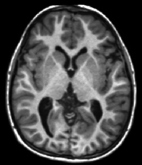
Figure 5.1: Magnetic Resonance Imaging (MRI) is an important application of image data in healthcare.

• Datasets of vectors. In practice, data is usually stored as vectors \(\vec x\in\mathbb{R}^m\). For example, the following graph illustrates data with \(m = 5\) (corresponding to “GDP per capita”, “life expectancy”, “name of country”, “population of country” and “date”).

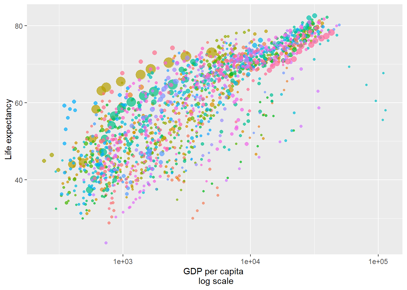
Figure 5.2: GDP data for different countries (each with its own colour) across time. Each dot represents a country on a specific date with the dot’s size corresponding to its population.

Therefore, we can represent a dataset of \(n\) vectors \(\{\vec x_1, \cdots, \vec x_n\}\) simply as an \(m\times n\) matrix, \[ X := \begin{bmatrix}\vec x_1 & \vec x_2 &\cdots & \vec x_n\end{bmatrix} = \begin{bmatrix}x_{1,1} & x_{2,1} & \cdots & x_{n,1}\\ x_{1,2} & x_{2,2} & \cdots & x_{n,2}\\ \vdots & \vdots & \ddots & \vdots\\ x_{1,m} & x_{2,m} &\cdots & x_{n,m} \end{bmatrix}. \] However, just as with images, it can be difficult to extract the key information from \(X\) (particularly if \(m\) and \(n\) are large). Thus, we are interested in dimensionality reduction and data compression more generally.

In this subsection, we will introduce the singular value decomposition (SVD) – which is widely considered to be the most important topic in numerical linear algebra. The SVD can be applied to any matrix, square or rectangular, and is the most prominent technique for matrix compression. Most notably, the SVD is used throughout data science for performing Principal Component Analysis (PCA).

Since the SVD has strong connections to symmetric eigenvalue problems, let us first recall the following theorem:

Theorem 5.8 (Symmetric eigenvalue decomposition) Let \(A\in\mathbb{R}^{n\times n}\) be a symmetric matrix. Then \(A\) admits the following matrix decomposition: \[\begin{equation} \tag{5.7} A = V\Lambda V^{\mathsf{T}}, \end{equation}\] where \(V\in\mathbb{R}^{n\times n}\) is orthogonal, \(V^{\mathsf{T}} V = I = VV^{\mathsf{T}}\), and \(\Lambda = \mathrm{diag}(\lambda_1, \cdots, \lambda_n)\) is a diagonal matrix of eigenvalues \(\lambda_i\in\mathbb{R}\).

In (5.7), \(\lambda_i\) are the eigenvalues and \(V\) is the matrix of eigenvectors (that is, its columns are eigenvectors).

It is worth noting that Theorem 5.8 is making two very strong claims. Namely, (a) the eigenvectors can be taken to be orthogonal and (b) the eigenvalues are real.

The decompoition (5.7) is not unique. We can always flip the sign of eigenvectors and if \(\lambda_i = \lambda_j\) for some \(i\neq j\), then the eigenvectors will span a subspace (whose dimension is the multiplicity of the eigenvalue). For example, any vector is an eigenvector of the identity matrix.

Before proceeding to our main theorem, we first recall the following key definitions.

Definition 5.8 The column rank of a matrix \(A = \begin{bmatrix}\vec a_1 &\cdots &\vec a_n\end{bmatrix}\in\mathbb{R}^{m\times n}\) is the dimension of its column space \(\mathrm{span}(\{\vec a_1, \cdots, \vec a_n\})\). Similarly, we can define the row rank of \(A\) as the dimension of its row space. It is a theorem that these ranks coincide and can thus unambiguously be called the rank of \(A\).

Definition 5.9 A matrix \(A\in\mathbb{R}^{m\times n}\) is said to have full rank if its rank equals \(\min(n,m)\).

We now present one of the most important results in numerical linear algebra – the Singular Value Decomposition. Note: we will only be proving this when \(A\) has full rank.

Theorem 5.9 (Singular Value Decomposition (SVD)) Let \(A\in\mathbb{R}^{m\times n}\) with \(m\geq n\). Then there exists \(U \in\mathbb{R}^{m\times m}\), \(\Sigma\in\mathbb{R}^{n\times n}\) and \(V\in\mathbb{R}^{n\times n}\) such that \[\begin{equation} \tag{5.8} A = U\begin{bmatrix}\Sigma \\ 0\end{bmatrix} V^{\mathsf{T}}, \end{equation}\] where \(U\) is orthogonal (i.e. \(U^\mathsf{T} U = UU^\mathsf{T} = I_m\)), \(V\) is orthogonal (i.e. \(V^\mathsf{T}V = VV^\mathsf{T} = I_n\)) and \(\Sigma = \mathrm{diag}(\sigma_1,\ldots, \sigma_n)\) with \(\sigma_1 \geq \sigma_2 \geq \cdots \geq \sigma_n \geq 0\).

Remark. The SVD easily applies to \(m\times n\) matrices with \(m < n\) simply by taking the transpose of (5.8). In a slight change of notation, it is more common to write the SVD (5.8) as \[\begin{equation} \tag{5.9} A = U\Sigma V^\mathsf{T}, \end{equation}\] where \(\Sigma\in\mathbb{R}^{m\times n}\) is still referred to as a diagonal matrix. However, the notation in (5.9) is much better suited for our proof.

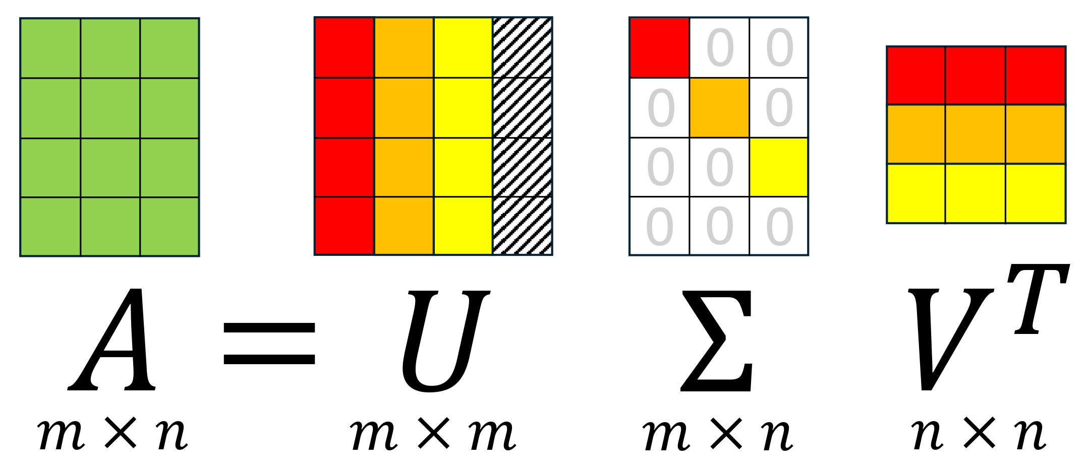
Figure 5.3: Visualisation of SVD. The hatched region corresponds to \(U_{⊥}\) in our proof.

Proof. (when \(A\) has full rank). Without loss of generality, we will assume that \(m\geq n\). This because if we had \(m < n\), then it would suffice to find an SVD for \(A^\mathsf{T}\) instead of \(A\).

Since \(A^\mathsf{T}A\) is symmetric, it admits an eigenvalue decomposition: \[ A^\mathsf{T}A = V\Lambda V^{\mathsf{T}}, \] where \(V\) is orthogonal.

Since \(A\) is assumed to have full rank, the null space of \(A\) is \(\{0\}\). Therefore, for an eigenvector \(\vec x\) and eigenvalue \(\lambda\) of \(A^\mathsf{T} A\), we have \(A\vec x \neq 0\) and \[ \|A\vec x\|_2^2 = (A\vec x)^\mathsf{T}(A\vec x) = \vec x^\mathsf{T} A^\mathsf{T} A \vec x = \lambda \|\vec x\|_2^2\,, \] which implies that \[ \lambda = \frac{\|A\vec x\|_2^2 }{\|\vec x\|_2^2} > 0. \] Hence, the diagonal of \(\Lambda\) must be positive – so we can write it as \(\Lambda = \Sigma^2\) where \(\Sigma\) is a positive diagonal matrix. Therefore, \(\Sigma^{-1}\) exists and we can define the matrix \(U_{\top} := AV\Sigma^{-1}\). This has orthogonal columns as \[ U_{\top}^{\mathsf{T}}U_{\top} = \Sigma^{-1}V^\mathsf{T}(A^\mathsf{T}A)V\Sigma^{-1} = \Sigma^{-1}(V^\mathsf{T} V)\Lambda (V^{\mathsf{T}}V)\Sigma^{-1} = I. \] Since the \(n\) columns of \(U_{\top}\) form an orthogonal basis for a subspace of \(\mathbb{R}^m\), we can use the Gram-Schmidt procedure to extend them to an orthogonal basis of \(\mathbb{R}^m\). Therefore, we can construct a matrix \(U_\bot\in\mathbb{R}^{m\times(m-n)}\) whose columns are these additional basis vectors.

We can now define the orthogonal matrix \(U := \begin{bmatrix} U_{\top} & U_{\bot}\end{bmatrix}\) and obtain the result as \(U_{\top}\Sigma V^\mathsf{T} = (AV\Sigma^{-1})\Sigma V^\mathsf{T} = A\).

Remark. The matrix \(U_\bot\) is often called the orthogonal complement of \(U_\top\). However, since it is multiplied by zeroes in the SVD (5.8), it has very little importance compared to \(U_\top\).

Finally, for the terminology “Singular Value Decomposition” to make sense, we will define the “Singular Values” of a matrix.

Definition 5.10 (Singular values and vectors) In Theorem 5.9, \(\{\sigma_i\}\) are called the singular values of \(A\). The columns of \(U = \begin{bmatrix}\vec u_1 & \vec u_2 & \cdots & \vec u_m\end{bmatrix}\) are called the left singular vectors and the columns of \(V = \begin{bmatrix}\vec v_1 & \vec v_2 & \cdots & \vec v_n\end{bmatrix}\) are called the right singular vectors.

Unsurprisingly, singular values are closely related to eigenvalues.

Theorem 5.10 Let \(\{\sigma_i\}\) denote the singular values of \(A\in\mathbb{R}^{m\times n}\). Then \[ \sigma_i = \sqrt{\lambda_i} \] where \(\{\lambda_i\}\) are the eigenvalues of \(A^\mathsf{T}A\) with \(|\lambda_1| \geq |\lambda_2| \geq \cdots |\lambda_n| \geq 0\). Furthermore,

• \(\{\lambda_i\}\) are the eigenvalues of \(AA^\mathsf{T}\),

• \(V = \begin{bmatrix} \vec v_1 & \cdots & \vec v_n\end{bmatrix}\) are the eigenvectors of \(A^\mathsf{T}A\),

• \(U = \begin{bmatrix} \vec u_1 & \cdots & \vec u_m\end{bmatrix}\) are the eigenvectors of \(AA^\mathsf{T}\).

Proof. From the Singular Value Decomposition (5.9), we have \[ A = U\Sigma V^\mathsf{T}. \] Therefore, the matrix \(A^\mathsf{T}A\) is \[ A^\mathsf{T}A = (U\Sigma V^\mathsf{T})^\mathsf{T}(U\Sigma V^\mathsf{T}) = V \Sigma \underbrace{U^{\mathsf{T}}U}_{=\, I_m}\Sigma V^\mathsf{T} = V \Sigma^2 V^\mathsf{T}, \] which is precisely the eigenvalue decomposition of \(A^\mathsf{T}A\). Therefore \(\Sigma^2\) are the eigenvalues of \(AA^\mathsf{T}\) and \(U\) gives the eigenvectors. An identical argument applies to \(AA^\mathsf{T}\) and gives the result.

The SVD tells us that any matrix can be written as orthogonal-diagonal-orthogonal. Roughly speaking, orthogonal matrices can be thought of as rotations or reflection, so the SVD says the action of a matrix can be thought of as a rotation/reflection followed by magnification (or shrinkage), followed by another rotation/reflection.

With this intuition, we would expect that the rank of \(A\) corresponds to rank of \(\Sigma\).

Theorem 5.11 The rank of \(A\) is equal to the number of positive singular values, \(\sigma_i > 0\).

Proof. We first note that, if \(A^\mathsf{T}A \vec x = 0\) where \(\vec x\in\mathbb{R}^n\), then \[ \|A\vec x\|_2^2 = (A\vec x)^\mathsf{T}(A\vec x) = \vec x^\mathsf{T}\big(A^\mathsf{T}A \vec x\big) = 0. \] Therefore \(A^\mathsf{T}A\) and \(A\) have the same null space. So by the rank-nullity theorem, they must have the same rank. From the SVD, we have \[ A^\mathsf{T}A = \big(V\Sigma^\mathsf{T} U^\mathsf{T}\big)\big(U\Sigma V^{\mathsf{T}}\big) = V\big(\Sigma^\mathsf{T}\Sigma\big) V^{\mathsf{T}}. \] The result now follows as the rank of the square matrix \(A^\mathsf{T}A\) equals the number of non-zero eigenvalues in \(\Sigma^\mathsf{T}\Sigma\).

Having covered quite a bit of theory, let’s consider an example.

Example 5.14 We would like to compute the SVD of the matrix \(A = \begin{bmatrix} -1 & -2 \\ 2 & 1 \\ 1 & 0 \\ 0 & 1\end{bmatrix}\).

Then the Gram Matrix is \(\,A^\mathsf{T}A = \begin{bmatrix}-1 & 2 & 1 & 0\\ -2 & 1 & 0 & 1\end{bmatrix}\begin{bmatrix} -1 & -2 \\ 2 & 1 \\ 1 & 0 \\ 0 & 1\end{bmatrix} = \begin{bmatrix} 6 & 4 \\ 4 & 6\end{bmatrix}\).

We can compute its eigenvalues as \(2\) and \(10\) using the characteristic polynomial \[ \mathrm{det}\bigg(\begin{bmatrix} 6 - \lambda & 4 \\ 4 & 6 - \lambda\end{bmatrix}\bigg) = 0 \Leftrightarrow (6 - \lambda)^2 = 16. \] Solving each eigenvalue problem yields the following eigenvector matrix, \[ V = \frac{1}{\sqrt{2}}\begin{bmatrix} 1 & - 1\\ 1 & 1\end{bmatrix}. \] Therefore \(A^\mathsf{T}A\) admits the eigenvalue decomposition, \[ A^\mathsf{T}A = V\Sigma^2 V^\mathsf{T}, \quad\text{where}\quad \Sigma^2 = \begin{bmatrix} 10 & 0\\ 0 & 2\end{bmatrix}. \] Hence \(U_{\top}\) can be computed as \[\begin{align*} U_{\top} = AV\Sigma^{-1} & = \begin{bmatrix} -1 & -2 \\ 2 & 1 \\ 1 & 0 \\ 0 & 1\end{bmatrix}\frac{1}{\sqrt{2}}\begin{bmatrix} 1 & - 1\\ 1 & 1\end{bmatrix}\begin{bmatrix} \frac{1}{\sqrt{10}} & 0 \\ 0 & \frac{1}{\sqrt{2}}\end{bmatrix}\\ & = \begin{bmatrix} -1 & -2 \\ 2 & 1 \\ 1 & 0 \\ 0 & 1\end{bmatrix}\begin{bmatrix} \frac{1}{\sqrt{20}} & - \frac{1}{2}\\ \frac{1}{\sqrt{20}} & \frac{1}{2}\end{bmatrix}\\ & = \begin{bmatrix} -\frac{3}{\sqrt{20}} & -\frac{1}{2}\\ \frac{3}{\sqrt{20}} & -\frac{1}{2}\\ \frac{1}{\sqrt{20}} & -\frac{1}{2}\\ \frac{1}{\sqrt{20}} & \frac{1}{2}\end{bmatrix}. \end{align*}\] Therefore, we have the following singular value decomposition for \(A\), \[ \begin{bmatrix} -1 & -2 \\ 2 & 1 \\ 1 & 0 \\ 0 & 1\end{bmatrix} = \left[\left.\begin{matrix} -\frac{3}{\sqrt{20}} & -\frac{1}{2}\\ \frac{3}{\sqrt{20}} & -\frac{1}{2}\\ \frac{1}{\sqrt{20}} & -\frac{1}{2}\\ \frac{1}{\sqrt{20}} & \frac{1}{2}\end{matrix}\,\,\right|\, U_\bot\right] \begin{bmatrix}\sqrt{10} & 0 \\ 0 & \sqrt{2} \\ 0 & 0 \\ 0 & 0\end{bmatrix}\begin{bmatrix} \frac{1}{\sqrt{2}} & \frac{1}{\sqrt{2}}\\ -\frac{1}{\sqrt{2}} & \frac{1}{\sqrt{2}}\end{bmatrix}, \] where the matrix \(U_{\bot}\) can be computed through the Gram-Schmidt procedure.

5.5.3 Low-rank approximation using the SVD

From the SVD (5.8) and Theorem 5.11, we obtain the following important alternative formula: \[\begin{equation} \tag{5.10} A = \sum_{i=1}^{\mathrm{rank}(A)}\sigma_i \vec u_i \vec v_i^\mathsf{T}, \end{equation}\] where \(\{\sigma_i\}\) are the singular values, \(U = \begin{bmatrix}\vec u_1 & \vec u_2 & \cdots & \vec u_n\end{bmatrix}\), \(V = \begin{bmatrix}\vec v_1 & \vec v_2 & \cdots & \vec v_n\end{bmatrix}\) and \(\mathrm{rank(A)}\) is precisely the number of non-zero \(\sigma_i\).

Letting \(R\) denote the rank of \(A\), we can visualise (5.10) as \[\begin{align*} A = \underbrace{\begin{bmatrix} \ast \\ \ast \\ \vdots \\ \ast\\ \ast\end{bmatrix}\begin{bmatrix} \ast & \ast & \cdots & \ast & \ast\end{bmatrix}}_{\sigma_1 \vec u_1 \vec v_1^\mathsf{T}} + \underbrace{\begin{bmatrix} \ast \\ \ast \\ \vdots \\ \ast\\ \ast\end{bmatrix}\begin{bmatrix} \ast & \ast & \cdots & \ast & \ast\end{bmatrix}}_{\sigma_2 \vec u_2 \vec v_2^\mathsf{T}} + \cdots + \underbrace{\begin{bmatrix} \ast \\ \ast \\ \vdots \\ \ast\\ \ast\end{bmatrix}\begin{bmatrix} \ast & \ast & \cdots & \ast & \ast\end{bmatrix}}_{\sigma_R \vec u_R \vec v_R^\mathsf{T}}. \end{align*}\]

Equation (5.10) reveals something quite interesting. It is possible to store the \(m\times n\) matrix \(A\) using only \(\mathrm{rank}(A)(m+n+1)\) numbers (since each triple \((\sigma_i, \vec u_i, \vec v_i)\) requires \(m+n+1\) numbers). As previously discussed, large matrices are ubiquitous throughout the sciences. So there is great interest in low-rank matrix approximation.

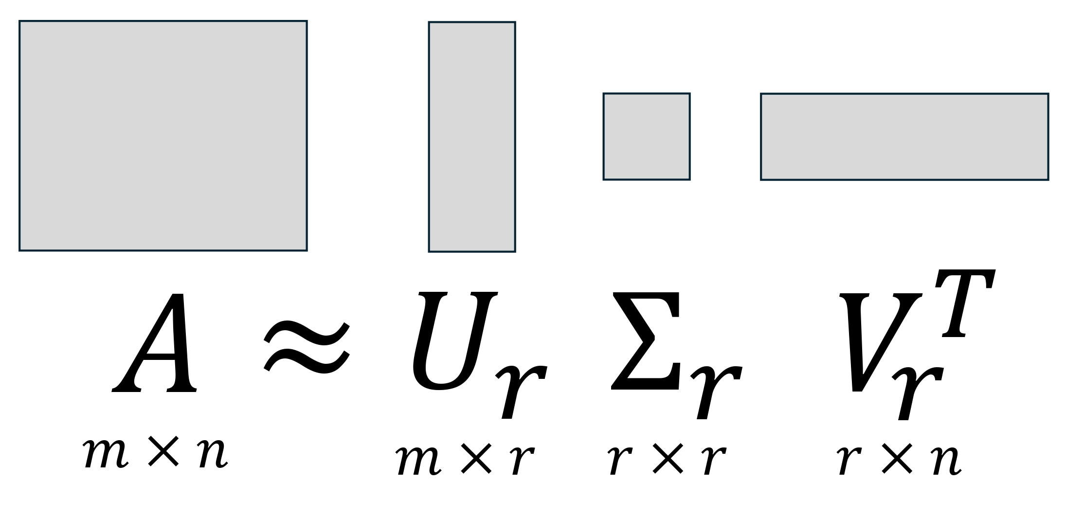
Figure 5.4: Visualisation of the low-rank approximation obtained by truncating SVD.

Definition 5.11 (Low-rank matrix approximation) Given a matrix \(A\in\mathbb{R}^{m\times n}\) with SVD (5.10), we define a rank-\(r\) approximation \(A_r\) as \[\begin{equation} \tag{5.11} A_r := \sum_{i=1}^r\sigma_i \vec u_i \vec v_i^\mathsf{T}. \end{equation}\] Alternatively, we can write \(A_r\) as \[ A_r = U_r \Sigma_r V_r^\mathsf{T}, \] where \(U_r = \begin{bmatrix}\vec u_1 & \vec u_2 & \cdots & \vec u_r\end{bmatrix}\in\mathbb{R}^{m\times r}\), \(V_r = \begin{bmatrix}\vec v_1 & \vec v_2 & \cdots & \vec v_r\end{bmatrix}\in\mathbb{R}^{n\times r}\) and \(\Sigma_r = \mathrm{diag}(\sigma_1,\cdots, \sigma_r)\).

Furthermore, due to the remarkable properties of SVD, matrix approximation via (5.11) is actually optimal in the following sense:

Theorem 5.12 (Optimality of matrix approximation using SVD) For any \(A\in\mathbb{R}^{m\times n}\) with singular values \(\sigma_1(A)\geq \sigma_2(A) \geq \cdots \geq \sigma_{\min(m,n)}(A)\geq 0\), and any non-negative integer \(r < \min(m,n)\), we have \[\begin{equation} \tag{5.12} \|A-A_r\|_2 = \sigma_{r+1}(A) = \min_{\mathrm{rank}(B)\leq r}\|A-B\|_2\,, \end{equation}\] where \(A_r\) is the rank-\(r\) approximation given by (5.11).

Proof. Not covered.

From this theorem, we can make a few observations:

• A good approximation \(A\approx A_r\) is achieved if and only if \(\sigma_{r+1} \ll \sigma_1\).

• Optimality actually holds under any norm that is invariant under multiplication by orthogonal matrices. We will not prove this optimality, but we can see that the Euclidean norm is invariant as \[\begin{equation} \tag{5.13} \|V\vec x\|_2^2 = (V\vec x)^\mathsf{T}(V\vec x) = \vec x^\mathsf{T} \underbrace{V^\mathsf{T} V}_{=\,I} \vec x = \|\vec x\|_2^2\,, \end{equation}\] for any orthogonal matrix \(V\in\mathbb{R}^{n\times n}\) and vector \(\vec x\in\mathbb{R}^n\). In particular, the above optimality theorem also holds under the Frobenius norm.

Definition 5.12 The Frobenius norm of a matrix \(A\in\mathbb{R}^{m\times n}\) is \[ \|A\|_F := \sqrt{\sum_{i=1}^m\sum_{j=1}^n |a_{ij}|^2} = \sqrt{\mathrm{tr}\big(A^\mathsf{T}A\big)}. \]

• A prominent application of low-rank approximation is PCA (Principal Component Analysis), which is often used in data science.

• By viewing a grayscale image as a matrix \(A\in\mathbb{R}^{m\times n}\), we can compute its SVD and visualise the resulting low-rank approximations. Whilst this is not the state of the art for image compression, it clearly demonstrates the effectiveness of SVD.

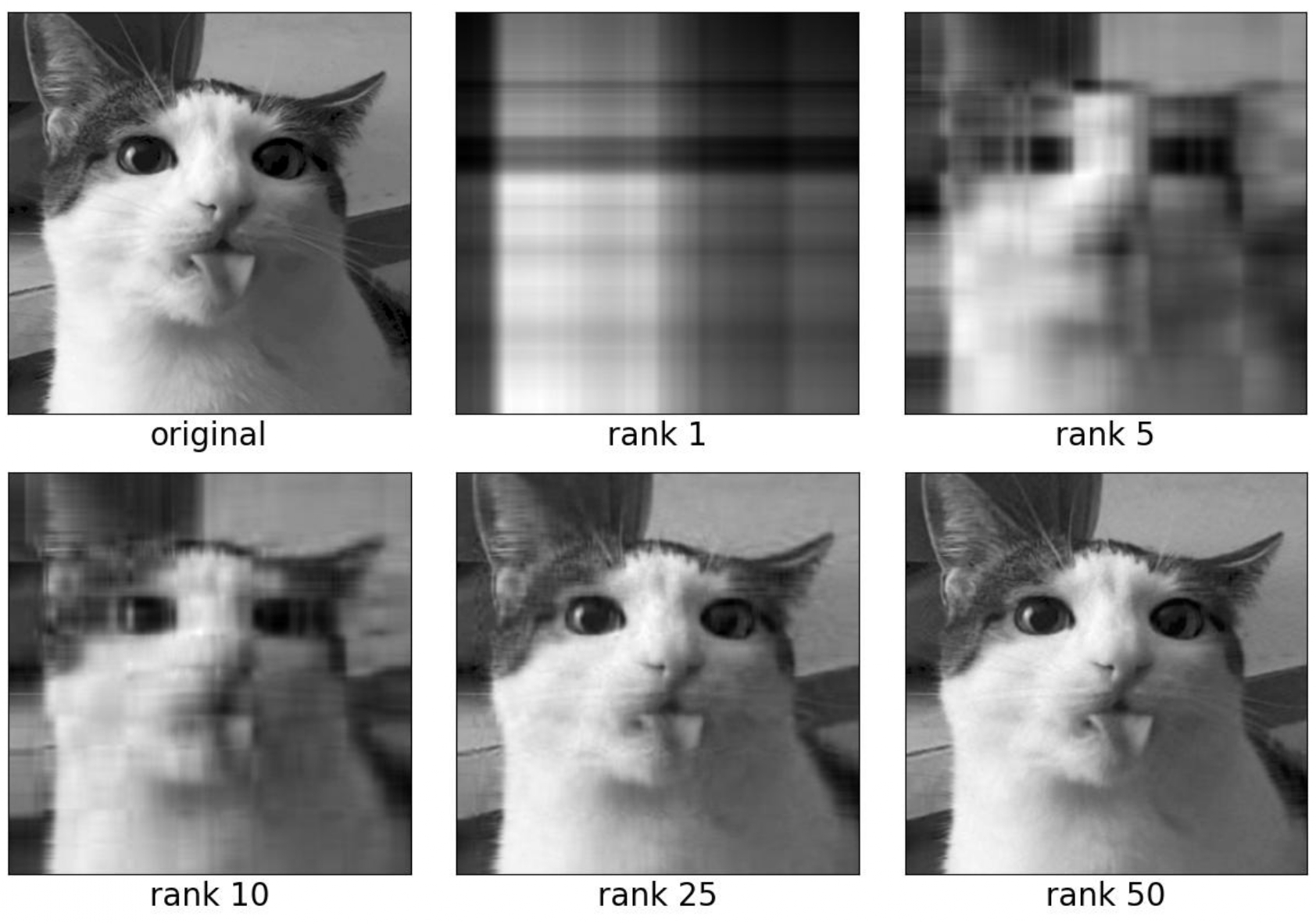
Figure 5.5: Image compression by low-rank approximation via the truncated SVD.

Although the proof of Theorem 5.12 is not covered, we will prove the following corollary.

Theorem 5.13 Let \(A\in\mathbb{R}^{m\times n}\). Then the first singular value of \(A\) is \[\begin{equation} \tag{5.14} \sigma_1 = \|A\|_2\,. \end{equation}\]

Proof. Without loss of generality, suppose \(m\geq n\).

Let \(\vec x\in\mathbb{R}^n\) be such that \(\|x\|_2 = 1\) and define \(\vec y := V^\mathsf{T} \vec x\). Then, since the Euclidean norm is invariant to multiplication by orthogonal matrices (see (5.13)), we have \(\|y\|_2 = 1\) and \[ \|A \vec x\|_2 = \|U\widetilde{\Sigma} V^\mathsf{T}\vec x\|_2 = \|U\widetilde{\Sigma} \vec y\|_2 = \|\widetilde{\Sigma} y\|_2\,, \] where \(\widetilde{\Sigma} := \begin{bmatrix}\Sigma\\ 0\end{bmatrix}\). Since \(\Sigma\) is an \(n\times n\) diagonal matrix, this gives \[ \|A \vec x\|_2 = \sqrt{\sum_{i=1}^n\sigma_i^2 y_i^2} \leq \sqrt{\sum_{i= 1}^n\sigma_1^2 y_i^2} = \sigma_1 \|\vec y\|_2 = \sigma_1 \|\vec x\|_2\,. \] Therefore, \(\|A\|_2 \leq \sigma_1\). On the other hand, taking \(\vec x = \vec v_1\) (the leading right singular vector), we obtain \(V^\mathsf{T}\vec v_1 = e_1\) and thus \(\|A\vec v_1\|_2 = \sigma_1\).

Figure 5.6: A geometric illustration for the SVD of a square matrix. In particular, we see that the leading singular value is the major semi-axis of the ellipse.

Finally, to conclude this section, we will discuss one of the most commonly used applications of SVD – dimensionality reduction.

That is, given data \(X = \{\vec x_1, \cdots, \vec x_n\} \subset \mathbb{R}^m\), we aim to compress it into a lower-dimensional space \(\mathbb{R}^{r}\) with \(r<m\) (ideally \(r \ll m\)). Perhaps the most common way to do this is to find a matrix \(W \in \mathbb{R}^{r \times m}\) that can reduce any \(\vec x \in X\) to \(\vec y := W \vec x \in \mathbb{R}^r\). Many computations can then be performed with the reduced vectors \(\vec y\) directly. However, to recover (or more precisely, approximate) the original data \(\vec z \approx \vec x\), we need another matrix \(U \in \mathbb{R}^{m \times r}\) such that \(\vec z = U \vec y\).

Definition 5.13 Given a dataset \(X = \{\vec x_1, \cdots, \vec x_n\}\subset\mathbb{R}^m\), the Principal Component Analysis (PCA) finds a compression matrix \(W_{\ast}\in\mathbb{R}^{r\times m}\) and a recovery matrix \(U_{\ast}\in\mathbb{R}^{m\times r}\) such that the mean squared error betweeen the recovered and original vectors in \(X\) is minimal, \[\begin{equation} \tag{5.15} W_{\ast}, U_{\ast} = \underset{W\in\mathbb{R}^{r\times m},\, U\in\mathbb{R}^{m\times r}}{\mathrm{arg}\,\mathrm{min}}\bigg(\frac{1}{n}\sum_{i=1}^n \big\|\vec x_i - UW \vec x_i\big\|_2^2\bigg)\,. \end{equation}\] The columns of \(U_{\ast}\) are called Principal Components.

Using the SVD, it is remarkably easy to solve the optimisation problem (5.15).

Theorem 5.14 The PCA problem (5.15) can be solved by taking \(U_\ast\) as the truncated matrix \(U_r = \begin{bmatrix}\vec u_1 & \vec u_2 & \cdots & \vec u_r\end{bmatrix}\in\mathbb{R}^{m\times r}\) from the SVD of \(X\) and \(W_{\ast} = U_{\ast}^\mathsf{T}\).

Proof. (non-examinable)

Let \(\vec y := W\vec x\in\mathbb{R}^r\) and \(Y = \begin{bmatrix}\vec y_1 & \cdots & \vec y_n\end{bmatrix}\in\mathbb{R}^{r\times n}\), then \[\begin{align*} \sum_{i=1}^n\big\|\vec x_i - UW \vec x_i\big\|_2^2 & = \sum_{i=1}^n\big\|\vec x_i - U\vec y_i\big\|_2^2\\ & = \sum_{i=1}^n\big(\vec x_i - U\vec y_i\big)^\mathsf{T}\big(\vec x_i - U\vec y_i\big)\\ & = \mathrm{tr}\big(\big(X - UY\big)^{\mathsf{T}}\big(X - UY\big)\big)\\ & = \big\|X - UY\big\|_F^2\,. \end{align*}\]

As \(\mathrm{span}(\{\vec y_1, \cdots, \vec y_n\})\) is a subspace of \(\mathbb{R}^r\), it is as most \(r\)-dimensional. This means that \(\{U \vec y : \vec y \in \mathrm{span}(\{\vec y_1, \cdots, \vec y_n\})\}\) must also be at most \(r\)-dimensional. However, since this is the column space of \(U Y\), it follows that \(\mathrm{rank}(UY)\leq r\).

So by the optimality of SVD, Theorem 5.12 (under the Frobenius norm), we see that the mean-squared error (5.15) is minimised when \[\begin{equation} \tag{5.16} UY = X_r\,, \end{equation}\] with \(X_r\) denoting the rank-\(r\) approximation of \(X\) given by \[ X_r = U_r \Sigma_r V_r^\mathsf{T}, \] where \(U_r = \begin{bmatrix}\vec u_1 & \vec u_2 & \cdots & \vec u_r\end{bmatrix}\in\mathbb{R}^{m\times r}\), \(V_r = \begin{bmatrix}\vec v_1 & \vec v_2 & \cdots & \vec v_r\end{bmatrix}\in\mathbb{R}^{n\times r}\) and \(\Sigma_r = \mathrm{diag}(\sigma_1,\cdots, \sigma_r)\) are obtained from the SVD of \(X\).

We claim that (5.16) is achieved by setting \(U = U_r\) and \(W = U_r^\mathsf{T}\). This can be shown by direct calculation, \[\begin{align*} U W X & = U_r U_r^\mathsf{T}X\\ & = U_r U_r^\mathsf{T}X_r + U_r U_r^\mathsf{T}(X - X_r)\\ & = U_r\,\underbrace{U_r^\mathsf{T}U_r}_{=\, I_m}\, \Sigma_r V_r^\mathsf{T} + U_r U_r^\mathsf{T}(X - X_r)\\ & = X_r + U_r U_r^\mathsf{T}(X - X_r). \end{align*}\]

Using the SVD formula (5.11) for \(X\) and \(X_r\), we can express their difference \(X - X_r\) as \[ X - X_r = \sum_{i\, \geq\, r+1}\sigma_i \vec u_i \vec v_i^\mathsf{T}. \] Therefore, for any \(j\leq r\), left multiplying by \(\vec u_j^\mathsf{T}\) gives \[ \vec u_j^\mathsf{T} (X-X_r) = \sum_{i\, \geq\, r+1}\sigma_i \big(\underbrace{\vec u_j^\mathsf{T} \vec u_i}_{=\,0}\big) \vec v_i^\mathsf{T} = 0, \] as \(\vec u_j\) and \(\vec u_i\) are orthogonal. Hence \(U_r^\mathsf{T}(X - X_r) = 0\) and \[ U W = X_r + U_r U_r^\mathsf{T}(X - X_r) = X_r\,, \] as required.

Remark. From Theorem 5.14, we see that the process of solving a PCA problem is exactly the same as obtaining the matrix \(U\) in the SVD. We note that if \(X = U\Sigma V^\mathsf{T}\) then \[ X X^\mathsf{T} = \big(U\widetilde{\Sigma} V^\mathsf{T}\big)\big(U\widetilde{\Sigma} V^\mathsf{T}\big)^\mathsf{T} = U\widetilde{\Sigma}\big(\underbrace{V^\mathsf{T} V}_{=\, I_n}\big)\widetilde{\Sigma}^\mathsf{T} U^\mathsf{T} = U\Sigma^2 U^\mathsf{T}, \] where \(\widetilde{\Sigma} := \begin{bmatrix}\Sigma\\ 0\end{bmatrix}\).

This is exactly the same as the symmetric eigenvalue decomposition given by Theorem 5.8. Therefore, to solve a PCA problem we can obtain the columns of \(U_r\) as the eigenvectors \(\vec u_1, \vec u_2, \cdots, \vec u_r\) of \(XX^\mathsf{T}\) corresponding to its largest \(r\) eigenvalues \(\sigma_1 \geq \sigma_2 \geq \cdots \geq \sigma_r\geq 0\).

To show that this gives us a practical way of computing PCA by hand, we shall present another example.

Example 5.15 Consider the following vectors in \(\mathbb{R}^2\), \[ \vec x_1 = \begin{bmatrix}1\\ -1\end{bmatrix},\quad\vec x_2 = \begin{bmatrix}-1\\ 1\end{bmatrix},\quad\vec x_3 = \begin{bmatrix}2\\ 2\end{bmatrix}, \] and suppose that we would like to reduce the dimension of the points \(\{\vec x_i\}\) to one.

Just as for SVD, we compute the (unnormalized) covariance matrix \(X X^\mathsf{T}\): \[\begin{align*} A = \sum_{i=1}^3 \vec x_i\vec x_i^\top & = \bigg(\begin{bmatrix}1\\ -1\end{bmatrix}\begin{bmatrix}1 & -1\end{bmatrix} + \begin{bmatrix}-1\\ 1\end{bmatrix}\begin{bmatrix}-1 & 1\end{bmatrix} + \begin{bmatrix}2\\ 2\end{bmatrix}\begin{bmatrix}2 & 2\end{bmatrix}\bigg)\\ & = \bigg(\begin{bmatrix} 1 & - 1\\ -1& 1\end{bmatrix} + \begin{bmatrix} 1 & - 1\\ -1& 1\end{bmatrix} + \begin{bmatrix} 4 & 4\\ 4 & 4\end{bmatrix} \bigg)\\ & = \begin{bmatrix} 6 & 2\\ 2 & 6\end{bmatrix}, \end{align*}\] Then the eigenvalues of \(A\) can be obtained by solving \[\begin{align*} \mathrm{det}\bigg( \begin{bmatrix} 6 - \lambda & 2\\ 2 & 6 - \lambda\end{bmatrix}\bigg) & = (6-\lambda)^2 - 4 = 0 \Leftrightarrow \lambda = 8\text{ or }4. \end{align*}\] Since \[\begin{align*} \begin{bmatrix} 6 & 2\\ 2 & 6\end{bmatrix}\begin{bmatrix} 1\\ 1\end{bmatrix} = 8\begin{bmatrix} 1\\ 1\end{bmatrix}, \end{align*}\] it follows that the leading eigenvector and the compression matrix are \[ W = U^\top = \frac{\sqrt{2}}{2}\begin{bmatrix} 1 & 1\end{bmatrix}. \] Therefore, the compressed data points (\(\vec y = W \vec x\)) are \[ \vec y_1 = 0,\quad\vec y_2 = 0,\quad\vec y_3 = 2\sqrt{2}, \] and the recovered data (\(\vec z = U \vec y\)) is \[ \vec z_1 = \begin{bmatrix}0\\ 0\end{bmatrix},\quad\vec z_2 = \begin{bmatrix} 0 \\ 0\end{bmatrix},\quad\vec z_3 = \begin{bmatrix}2\\ 2\end{bmatrix}. \] As a nice exercise, you could plot the original data points (\(\vec x_1, \vec x_2, \vec x_3\)) are consider why the PCA would map them to (\(\vec z_1, \vec z_2, \vec z_3\)) .

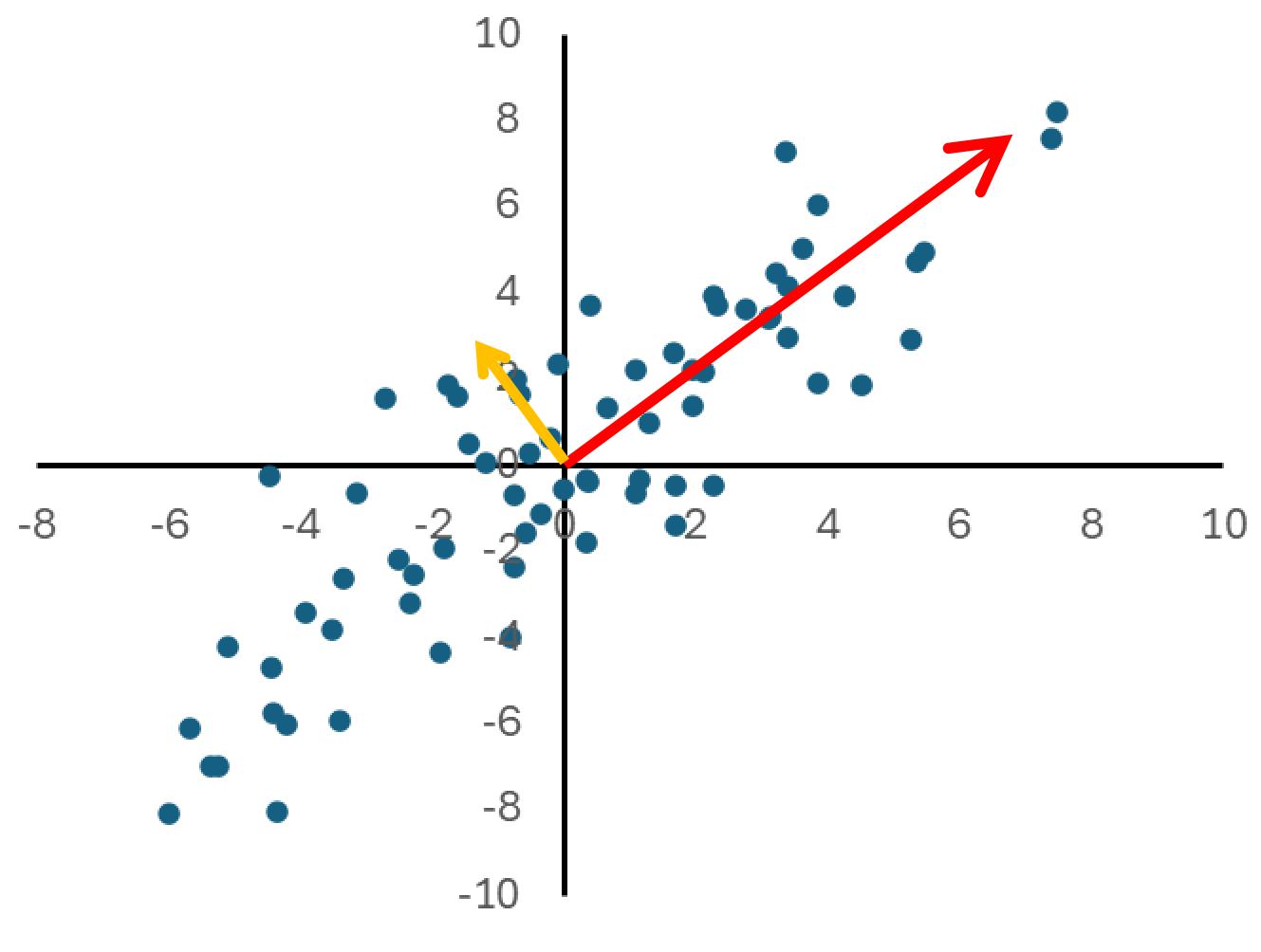
Figure 5.7: The principal components are the directions which explain the variance of the data.