Chapter 3 Numerical integration

Problem. Given a function \(f: [a,b]\to \mathbb{R}\), compute approximations of \(\int^b_a f(x)\,dx\) using only samples of \(f\) at some points in the interval \([a,b]\).

Numerical integration is important since, for many functions \(f\), the integral cannot be found exactly, but point values of \(f\) are relatively easy to compute (e.g., \(f(x)= \exp(x^2)\)). Initially, we work on a reference interval \([a,b]=[0,1]\) and consider first

\[\begin{equation} \int^1_0 f(x)\,dx. \tag{3.1} \end{equation}\] We approximate this by quadrature rules of the form \[\begin{equation} Q(f) = \sum^{N}_{i=0}w_if(x_i) \tag{3.2} \end{equation}\] where \(x_i\) are distinct points in \([0,1]\) and \(w_i\) are some suitable weights. We study ways to fix the \(x_i\) and the \(w_i\) independently of any particular choice of \(f\), so that (3.2) can be computed easily for any \(f\).
How to choose \(x_i\) and \(w_i\)?

Idea: Replace \(f\) with an interpolating polynomial. Polynomials are simple to integrate and lead to easy-to-use quadrature rules with a set of weights \(w_i\) for any given set of points \(x_i\).

3.1 Newton-Cotes rules

3.1.1 Newton-Cotes rules over the interval \([0,1]\)

Start with equally spaced points \(x_i= {i}/{N}\,, i = 0, \ldots, N,\) and find suitable weights \(w_i\). We construct the rule (3.2) by integrating the degree-\(N\) interpolating polynomial \(p_N(x)\) for \(f\) at \(x_i\).

Two points: For \(N=1\), we have two points \(x_0=0\) and \(x_1=1\). Then (see Section 2), the linear interpolant to \(f\) is \[ p_1(x) =f(0)+(f(1)-f(0)) \, x \] and \[\begin{align*} \int^1_0 p_1(x)\,dx &= f(0)+(f(1)-f(0)) \int^1_0 x\,dx \\ &= f(0)+\frac12(f(1)-f(0)) = \frac12 \left({ f(0)+f(1)}\right). \end{align*}\] We have derived the trapezoidal or trapezium rule \[\begin{equation} \tag{3.3} Q_1(f) := \frac12 \left({ f(0)+f(1)}\right) \quad \text{for approximating}\quad \int^1_0f(x)dx. \end{equation}\] Here the weights \(w_0 = w_1 = \frac12\,\). It is called the trapezium rule because it approximates \(\int^1_0f(x)\,dx\) by the area of the trapezium under the straight line \(p_1(x)\) that interpolates \(f\) between \(0\) and \(1\). It is exact (i.e., \(Q_1(f) = \int_0^1 f(x)\,dx\)) for any polynomial \(f\) of degree \(1\) (i.e., \(f \in \mathcal{P}_1\)), since in that case \(p_1 = f\) by the uniqueness of the linear interpolant (recall Theorem 2.2).

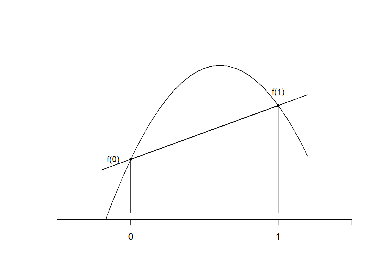
Figure 3.1: The trapezium rule

For \(N=2\), we have three points \(x_0=0\), \(x_1=1\), and \(x_2=1/2\). Using the Newton divided-difference form of the quadratic interpolant, \[\begin{equation*} p_2(x) = f(0)+f[0,1]x+ f[0,1,1/2]x(x-1). \end{equation*}\] Then, \[\begin{align*} \int^1_0 p_2(x)\,dx & = f(0) + \frac12 f[0,1] +f[0,1,1/2] \underbrace{\int^1_0 (x^2-x)\,dx}_{= -1/6}\\ &= f(0) + \frac12 \frac{f(1)-f(0)}1 - \frac16 \frac{f[0,1/2]-f[0,1]}{1/2-1}, \end{align*}\] where \(f[0,1/2]=2(f(1/2)-f(0))\) and \(f[0,1]=f(1)-f(0)\). Thus, \[\begin{align*} \int^1_0 p_2(x)\,dx &= f(0) + \frac12 (f(1)-f(0)) +\frac13 \left({ 2f(1/2)-2f(0)+f(0)-f(1)}\right)\\ &= \frac16\left[{f(0)+4f\left({\textstyle \frac12}\right)+f(1)}\right]. \end{align*}\] This is called Simpson’s rule. We write \[\begin{equation} \tag{3.4} Q_2(f) := \frac16f(0)+ \frac46 f\left({\textstyle \frac12}\right)+ \frac16f(1), \end{equation}\] with weights \(w_0 = w_1 = \frac{1}{6}\) and \(w_2 = \frac{4}{6}\). This rule is exact for all \(f \in \mathcal{P}_2\), since again in that case \(p_2 = f\).

In general, Newton-Cotes quadrature rules are of the form \[ Q_N(f) := \sum^N_{i=0}w_if(x_i) \] where \(x_i= i/N\) for \(i=0,\dots,N\), and the weights \(w_i\) can be found by integrating the degree-\(N\) interpolating polynomial. By writing \(p_N(x)\) using the Lagrange basis functions (see the proof of Theorem 2.2), \[ p_N(x)=\sum_{i=0}^N L_i(x) f(x_i), \] we can show that \[ w_i=\int_0^1 L_i(x)\,dx. \]

3.1.2 Newton-Cotes rules over a general interval \([a,b]\)

Suppose now we have a rule \[\begin{equation} \tag{3.5} Q(f) = \sum_{i=0}^N w_i f(x_i)\quad \quad \text{that approximates} \quad \quad \int_0^1 f(x) \,dx. \end{equation}\] To approximate \(\int_a^b f(t) dt\), we make a change of variable \(\displaystyle x = \frac{t-a}{b-a}\) and \(dx=\frac{1}{b-a}dt\). Then, \(t \in [a,b]\) is mapped to \(x\in [0,1]\) and \[ \int^b_a f(t) \,dt =\int^1_0 \underbrace{(b-a)f\left({a+x(b-a)}\right)}_{\textstyle =: g(x)}\,dx = \int_0^1 g(x) \,dx. \]

We now use \(Q(g)\) to approximate the right-hand side, to obtain the rule \[\begin{equation} Q^{[a,b]}(f) := \sum_{i=0}^N w_i g(x_i) = (b-a) \sum_{i=0}^N w_i f\left({a + (b-a) x_i}\right). \tag{3.6} \end{equation}\]

Notation: We use superscript \([a,b]\) to denote a rule over \([a,b]\). We omit the superscript for \([0,1]\). The lowest-order Newton-Cotes rules on a general interval \([a,b]\) are \[\begin{alignat*}{2} Q_{1}^{[a,b]}(f) & = \frac{b-a}{2} \left({f(a) + f(b)}\right), &\text{trapezium rule}\\ Q_{2}^{[a,b]}(f) & = \frac{b-a}{6} \left({f(a) + 4 f\left({\frac{b + a}{2}}\right) + f(b)}\right), \qquad &\text{Simpson's rule.} \end{alignat*}\]

Example 3.1 Let us apply these to the integral of \(f(x) = \sqrt{x}\) over \([1/4,1]\). Then \[ Q_1^{[1/4,1]} (f) = \frac{1 - \frac{1}{4}}{2} \left({\sqrt{1/4} + 1}\right) = \frac{3}{8} \, \frac{3}{2} = 9/16 = 0.5625, \qquad\quad \text{trapezoidal} \] \[ Q_2^{[1/4,1]} (f) = \frac{1 - \frac{1}{4}}{6} \left({\sqrt{1/4} + 4 \sqrt{5/8} + 1}\right) =0.582785\quad\text{(6 s.f.),} \quad \text{Simpson's.} \] The exact value \[ \int^1_{1/4}\sqrt{x}\,dx = \frac{2}{3} \left[{x^{3/2}}\right]_{1/4}^1 = \frac{7}{12} = 0.583333\quad \text{(6 s.f.)}, \] so the absolute value of the error in Simpson’s rule is \(\lvert{ 0.582785 - 0.583333 }\rvert = 5.48 \times 10^{-4}\), which is about 38 times smaller than the error in the trapezoidal rule \(\lvert{ 9/16 - 0.583333 }\rvert = 2.083\times 10^{-2}\).

3.1.3 Composite rules

As for the piecewise interpolation in 2, instead of increasing the accuracy of quadrature by choosing higher-order interpolating polynomials, we can also split the integration domain into subintervals by introducing a mesh and applying low-order rules on the sub-intervals.

Consider a general quadrature rule (e.g., from Section 3.1) \[\begin{equation} \tag{3.7} Q(f) = \sum_{i=0}^N w_if(x_i) \quad \text{that approximates} \quad \int^1_0f(x)\,dx, \end{equation}\] for some \(N\), weights \(w_i\) and distinct points \(x_i\). To approximate \(\int_a^b f(t)\, dt\), we introduce the mesh \(a = y_0 < y_1 < \cdots < y_J = b\) and write \[ \int_a^b f(t)\, dt = \int_{y_{0}}^{y_1} f(t) \, dt + \int_{y_{1}}^{y_2} f(t) \, dt + \cdots + \int_{y_{J-1}}^{y_J} f(t) \, dt = \sum_{j=1}^J \int_{y_{j-1}}^{y_j} f(t) \, dt. \] Now use the quadrature rule given by (3.7) on each subinterval, to obtain the approximation \[\begin{equation} \int_a^b f(t) \,dt \approx \sum_{j=1}^J Q^{[y_{j-1}, y_j]} (f) = \sum_{j=1}^J h_j \sum_{i=0}^N w_i f(y_{j-1}+h_jx_i), \tag{3.8} \end{equation}\] where \(h_j = y_j - y_{j-1}\). The approximation (3.8) is known as the composite version of (3.7).

As in the case of interpolation, we expect that accuracy will increase when the mesh width \(\max_j h_j \rightarrow 0\).

Example 3.2 (composite trapezoidal rule)   \[\begin{equation} \tag{3.9} Q_{1,J}^{[a,b]}(f) := \sum_{j = 1}^J Q_1^{[y_{j-1},y_j]}(f) = \sum_{j=1}^J\frac{h_j}{2}\left({f(y_{j-1})+f(y_j)}\right). \end{equation}\] For a uniform mesh, \(h_j = h := (b-a)/J\),, \(j=1,\ldots,J\), this can be written compactly as \[ Q_{1,J}^{[a,b]}(f) := h \left({ \frac{f(a)}{2} + \sum_{j=1}^{J-1} f(y_j) \; + \; \frac{f(b)}{2} }\right). \]

Example 3.3 (composite Simpson's rule)   \[\begin{equation} \tag{3.10} Q_{2,J}^{[a,b]}(f) := \sum_{j=1}^J Q_2^{[y_{j-1}, y_j]}(f) = \sum_{j=1}^J\frac{h_j}{6}\left({f(y_{j-1})+4f(m_j) + f(y_j)}\right), \end{equation}\] where the midpoints \(\displaystyle m_j = \frac{y_{j-1} + y_j}{2}\). For a uniform mesh, this can again be written more compactly as \[ Q_{2,J}^{[a,b]}(f) =\frac{h}{6}\left[{ f(a) + 2 \sum_{j=1}^{J-1}f(y_j) + 4 \sum_{j=1}^{J} f(m_j) + f(b) }\right]. \]

Please implement the general formulae (3.9) and (3.10) in Python, so that we can apply the rules on any mesh.

3.2 Error analysis

3.2.1 Non-composite rules over \([0,1]\)

Given a rule \[\begin{equation} \tag{3.11} Q(f) := \sum_{i=0}^N w_if(x_i) \end{equation}\] that approximates \[I(f) := \int^1_0f(x)\,dx,\] we define the error in the quadrature rule to be \[\begin{equation} \tag{3.12} E(f) := I(f) - Q(f) \; . \end{equation}\]

Definition 3.1 (DoP) The rule \(Q(f)\) in (3.11) has degree of precision (DoP) \(d\in\mathbb{N}\) if

\[ E(x^r)=0 \quad \text{ for all $r\in\mathbb{N}$ with $0\le r \leq d, \qquad$ and $E(x^{d+1}) \ne 0$.} \]

Example 3.4 (trapezium rule DoP) The trapezium rule \(Q_1(f)=\frac12(f(0)+f(1))\), and the error \(E_1(f) := I(f)-Q_1(f)\). We create the following table:

\(r\)	\(x^r\)	\(I(x^r)\)	\(Q_1(x^r)\)	\(E_1(x^r)\)
0	1	1	\(\frac12\cdot 1 + \frac12\cdot 1 = 1\)	0
1	\(x\)	\(\frac12\)	\(\frac12\cdot 0 + \frac12\cdot 1 = \frac12\)	0
2	\(x^2\)	\(\frac13\)	\(\frac12\cdot 0 + \frac12\cdot 1 = \frac12\)	\(-\frac16\)

Hence the DoP of the trapezoidal rule is \(1\).

Example 3.5 (Simpson's rule DoP) Simpson’s rule \(Q_2(f)=\frac16 \left[ {f(0)+4f\left(\frac12\right)+f(1)} \right]\), and the error \(E_2(f) := I(f)-Q_2(f)\). We create the following table:

\(r\)	\(x^r\)	\(I(x^r)\)	\(Q_2(x^r)\)	\(E_2(x^r)\)
0	1	1	\(\frac16\left(1\cdot 1 + 4\cdot 1 + 1\cdot 1\right) = 1\)	0
1	\(x\)	\(\frac12\)	\(\frac16\left(1\cdot 1 + 4\cdot \frac12 + 1\cdot 1\right) = \frac12\)	0
2	\(x^2\)	\(\frac13\)	\(\frac16\left(1\cdot 1 + 4\cdot \left(\frac12\right)^2 + 1\cdot 1\right)= \frac13\)	0
3	\(x^3\)	\(\frac14\)	\(\frac16\left(1\cdot 1 + 4\cdot \left(\frac12\right)^3 + 1\cdot 1\right)= \frac14\)	0
4	\(x^4\)	\(\frac15\)	\(\frac16\left(1\cdot 1 + 4\cdot \left(\frac12\right)^4 + 1\cdot 1\right)= \frac{5}{24}\)	\(-\frac{1}{120}\)

Hence the DoP of Simpson’s rule is \(3\).

The trapezium rule \(Q_1\) is found by integrating \(p_1\) and it is not surprising that its DoP is 1. Similarly, \(Q_2\) is found by integrating \(p_2\) and thus we’d expect a DoP of at least 2. A DoP of \(3\) is a surprise.
In fact, it turns out that for all \(N \in \mathbb{N}\) the Newton-Cotes rule \(Q_N(f)\) is of DoP \(N\) if \(N\) is odd and of DoP \(N+1\) if \(N\) is even.

Proposition 3.1 If (3.11) has DoP \(d\), then \[ E(p) = 0,\quad \text{for all} \quad p\in \mathcal{P}_d. \]

Proof. For any \(f_1, f_2: [0,1]\to \mathbb{R}\) and \(\alpha,\beta\in\mathbb{R}\), \[\begin{equation} \tag{3.13} I(\alpha f_1+\beta f_2)\; =\; \alpha I(f_2)+\beta I(f_2)\quad\text{and}\quad Q(\alpha f_1+\beta f_2) \; = \; \alpha Q(f_2)+\beta Q(f_2), \end{equation}\] since \(I\) and \(Q\) are both linear transformations.

If \(p\in\mathcal{P}_d\), \(p\) is a polynomial of degree less than or equal to \(d\) and can be written \[ p(x)=\sum^d_{r=0}a_rx^r,\quad\text{for some coefficients }\, a_r \in \mathbb{R}. \] Hence, using (3.13), \[ I(p)-Q(p) = \sum^d_{r=0} a_r \left[{I(x^r)-Q(x^r) }\right] = 0, \] since the DoP equals \(d\).

With significant further work, we can show that, for the trapezium rule, there exists \(\xi\in[0,1]\) such that \[\begin{equation} \tag{3.14} E_1(f) = \left[{ \frac{E_1(x^2)}{2!}}\right] f''(\xi) = - \frac{1}{12} f''(\xi), \qquad \text{for all} \ f \in C^2[0,1]. \end{equation}\] For \(p\in \mathcal{P}_1\), \(p''\equiv 0\) and \(E_1(p)=0\) as expected from the DoP calculation.

For Simpson’s rule, there exists \(\xi\in[0,1]\) such that \[ E_2(f)= \left[{\frac{E_2(x^4)}{4!}}\right]f^{(\mathrm{4})}(\xi) = - \frac{1}{2880} f^{(\mathrm{4})}(\xi), \qquad \text{for all} \ f \in C^4[0,1]. \] Notice the error for Simpson’s rule depends on the fourth derivative of \(f\) while that for the trapezium rule depends on the second derivative. Here \(C^k[a,b]\) is the set of functions \(f: [a,b]\to \mathbb{R}\) that are \(k\)-times continuously differentiable.

This leads to estimates over \([a,b]\) instead of \([0,1]\) by a change of variables.

Example 3.6 The error for the trapezoidal rule over \([a,b]\) is \[ E_1^{[a,b]} (f) := \int_a^b f(t)\, dt - Q_1^{[a,b]}(f). \] To determine the error, we recall that \[ \int_a^b f(t) \,dt =\int_0^1 g(x)\,dx,\qquad Q_1^{[a,b]}(f)=Q_1(g), \] from (3.6) with \(g(x)=(b-a) f(a+(b-a)x)\). Now \(g'(x)=(b-a)^2 f'(a+(b-a)x)\) and \(g''(x)=(b-a)^3 f''(a+(b-a)x)\). By (3.14), \[ E_1(g) = \int_0^1 g(x)\,dx - Q_1(g)=-\frac{1}{12}g''(\xi)=-\frac{1}{12} (b-a)^3 f''(\eta) \] for some \(\xi\in[0,1]\) and \(\eta:= a+(b-a)\xi\). Then, \[ E_1^{[a,b]} (f) = - \frac{(b-a)^3}{12} f''(\eta) \quad \quad \text{ for some} \quad \eta \in [a,b]. \] A similar calculation shows that the error for Simpson’s rule over \([a,b]\) is \[ E_2^{[a,b]} (f) := \int_a^b f (t) \,dt - Q_2^{[a,b]}(f) = - \frac{(b-a)^5}{2880} f^{(4)}(\eta) \qquad \text{ for some $\eta \in [a,b]$.} \] Notice the fifth power of \((b-a)\), which comes from the change of coordinates from \(t\) to \(x\).

3.2.2 Composite Newton-Cotes rules

Let \(Q_N\) be a Newton-Cotes rule on \([0,1]\) with degree of precision \(d\). The composite version with \(J\) subintervals on \([a,b]\) is (as in Section 3.1.3): \[ Q_{N,J}^{[a,b]}(f) = \sum_{j=1}^J Q_N^{[y_{j-1},y_j]}(f). % \] The error can be expressed in terms of the error made in approximating the sub-integrals. \[ E_{N,J}^{[a,b]}(f) := \int_a^b f(x) \,dx - Q_{N,J}^{[a,b]}(f) = \sum_{j=1}^J \underbrace{\left[{ \int_{y_{j-1}}^{y_j} f(x)\,dx - Q_N^{[y_{j-1},y_j]}(f)}\right]}_{=E_N^{[y_{j-1},y_j]}(f)}. \] We have formula for \(E_N^{[a,b]}\) for \(N=1,2\), which lead to the following error estimates for the composite trapezium and Simpson’s rule.

Example 3.7 (Composite trapezium rule error) If \(f \in C^2[a,b]\), then there exists \(\eta_j \in [y_{j-1},y_j]\) such that \[ E_{1,J}^{[a,b]} (f) = - \frac{1}{12} \sum_{j=1}^J h^{3}_j f^{(2)}(\eta_j) \qquad \text{and} \qquad \big|E_{1,J}^{[a,b]}(f)\big| \le \frac{b-a}{12} \lVert{ f^{(2)} }\rVert_{\infty,[a,b]} h^2, \] since \(\sum_{j=1}^J h_j=b-a\).

Example 3.8 (Composite Simpson's rule error) If \(f \in C^4[a,b]\), then there exists \(\eta_j \in [y_{j-1},y_j]\) such that \[ E_{2,J}^{[a,b]} (f) = - \frac{1}{2880} \sum_{j=1}^J h^{5}_j f^{(4)}(\eta_j) \qquad \text{and} \qquad \big|E_{2,J}^{[a,b]} (f)\big| \le \frac{b-a}{2880} \lVert{ f^{(4)} }\rVert_{\infty,[a,b]} h^4. \]

If \(f(x)\) fails to be sufficiently differentiable on all of \([a,b]\), but is sufficiently differentiable on subintervals of \([a,b]\), we can apply error estimates there.

Example 3.9 Consider \(f(x) = \sqrt{x}\) on \([0,1]\), which has infinitely many derivatives on subintervals that do not contain~\(0\), but no bounded derivatives on \([0,1]\). Consider the composite trapezoidal rule for \(\int_0^1 f(x) \,dx\) on the mesh \(0=y_0 < y_1 < \cdots < y_J=1\). Then \[\begin{align} E_{1,J}^{[0,1]} (f) = & E_{1,J}^{[0,y_1]} (f) + E_{1,J}^{[y_1,1]} (f) \nonumber \\ = & \left({ \int_0^{y_1} f(x) \, \,dx - h_1 \frac{\sqrt{y_1}}{2} }\right) - \frac{1}{12} \sum_{j=2}^J h_j^{3} f^{(2)}(\eta_j)\;. \tag{3.15} \end{align}\] Now, we can estimate each of the terms in (3.15) separately (see Problem E5.2).

3.3 Gaussian quadrature rules

The only examples of quadrature rules so far have been Newton-Cotes rules with equally spaced points. Can we do better with other points?

To take advantage of symmetry and simplify calculations, we work on the interval \([-1,1]\) rather than \([0,1]\) (which can of course be transformed onto \([0,1]\)). Let \(x_i\), \(i=0,\dots,N\), be arbitrary points in \([-1,1]\), and let \(p_N(x)\) be the degree-\(N\) interpolating polynomial for a function \(f\) at these points. Consider the rule:

\[\begin{equation} \tag{3.16} Q_{\mathrm{Gauss},N}^{[-1,1]}(f):= \int^1_{-1}p_N(x)\,dx \end{equation}\] as an approximation to \[\begin{equation} \tag{3.17} \int^1_{-1}f(x)\,dx. \end{equation}\] This rule has DoP at least \(N\). Can we do better with a clever choice of points? There are \(2N+2\) degrees of freedom (given by choice of \(x_i\) and \(w_i\) for \(i=0,\dots,N\)) and \(d+1\) conditions to achieve of a DoP of \(d\). By equating the number of conditions to the number of degrees of freedom, \(d+1=2N+2\), we hope that a DoP \(d=2N+1\) can be achieved by careful choice of \(x_i\) and weights \(w_i\).

Example 3.10 (One point, N=0) To achieve a DoP of \(d=2N+1=1\), we demand that \[\begin{equation} \tag{3.18} Q(1) = \int_{-1}^1 1\,dx=2\qquad\text{and}\qquad Q(x) =\int_{-1}^1 x\,dx=0. \end{equation}\] As \(p_0(x)\) is a constant, we must have \(p_0(x)=f(x_0)\) and \[ Q(f)=w_0 f(x_0). \] Then, \(w_0=2\) and \(x_0=0\) gives (3.18). Therefore, the one-point Gauss rule (or midpoint rule), obtained by integrating the degree-0 interpolant \(p_0\) at \(x_0=0\) over \([-1,1]\) is \[\begin{align*} Q_{\mathrm{Gauss},0}^{[-1,1]}(f) := \int^1_{-1} p_0(x)\,dx = 2 f(0). \end{align*}\] This is exact when \(f=1\) and \(f=x\), so it is a one-point rule with DoP \(=1\). Any other one-point rule has only DoP \(=0\).

Example 3.11 (Two points, N=1) To achieve a DoP \(d=2N+1=3\), we demand that \[ Q(1)=2,\qquad Q(x)=0, \qquad Q(x^2)=\frac{2}{3},\qquad\text{and}\qquad Q(x^3)=0. \] As \[ Q(f)= w_0 f(x_0)+w_1 f(x_1), \] we must have \(w_0+w_1=2\) and \(w_0 x_0 +w_1 x_1=0\) and \(w_0 x_0^2+w_1 x_1^2=2/3\) and \(w_0 x_0^3+ w_1 x_0^3=0\). By symmetry considerations, we must have \(x_0=-x_1\) and \(w_0=w_1\). Then \(w_0=w_1=1\) and \(2 x_0^2=2/3\), so that \(x_0=\sqrt{1/3}\). We obtain the two-point Gauss rule \[\begin{align*} Q_{\mathrm{Gauss},1}^{[-1,1]}(f) := \int^1_{-1} p_1(x)\,dx = f\left({\frac{1}{\sqrt3}}\right) + f\left({-\frac{1}{\sqrt3}}\right). \end{align*}\] Although only a two-point rule, its DoP is \(2N +1 = 3\). Compare with the trapezium rule which uses two points and has DoP only \(1\)!

Remark. Composite Gauss rules can also be derived and are highly effective.

High-frequency integrands, where \(f\) oscillates rapidly and where the derivatives of \(f\) are large, are particularly difficult and arise, for example, in high-frequency scattering applications (e.g., radio waves). This requires special techniques such as Filon quadrature.

Multivariate integrals are also important. For low-dimensional problems, simple tensor-product rules (applying one-dimensional rules in each dimension) work fine and our theory carries over easily. For high-dimensional integrals, the only feasible methods currently are Monte Carlo-type methods.