Chapter 3 Numerical integration

Problem Given a function \(f\colon [a,b]\to \mathbb{R}\), compute approximations of \(\int^b_a f(x)\,dx\) using only samples of \(f\) at some points in the interval \([a,b]\).

Numerical integration is important since, for many functions \(f\), the integral cannot be found exactly, but point values of \(f\) are relatively easy to compute (e.g., \(f(x)= \exp(x^2)\)). Initially, we work on a reference interval \([a,b]=[0,1]\) and consider first

\[\begin{equation} \int^1_0 f(x)\,dx. \tag{3.1} \end{equation}\] We approximate this by quadrature rules of the form \[\begin{equation} Q(f) = \sum^{N}_{i=0}w_if(x_i) \tag{3.2} \end{equation}\] where \(x_i\) are distinct points in \([0,1]\) and \(w_i\) are some suitable weights. We study ways to fix the \(x_i\) and the \(w_i\) independently of any particular choice of \(f\), so that (3.2) can be computed easily for any \(f\).
How to choose \(x_i\) and \(w_i\)?

Idea: Replace \(f\) with an interpolating polynomial. Polynomials are simple to integrate and lead to easy-to-use quadrature rules with a set of weights \(w_i\) for any given set of points \(x_i\).

3.1 Newton–Cotes rules

3.1.1 Newton–Cotes rules over the interval \([0,1]\)

Start with equally spaced points \(x_i= {i}/{N}\,, i = 0, \ldots, N,\) and find suitable weights \(w_i\). We construct the rule (3.2) by integrating the degree-\(N\) interpolating polynomial \(p_N(x)\) for \(f\) at \(x_i\).

Two points: For \(N=1\), we have two points \(x_0=0\) and \(x_1=1\). Then (see Section 2), the linear interpolant to \(f\) is \[ p_1(x) =f(0)+(f(1)-f(0)) \, x \] and \[\begin{align*} \int^1_0 p_1(x)\,dx &= f(0)+(f(1)-f(0)) \int^1_0 x\,dx \\ &= f(0)+\frac12(f(1)-f(0)) = \frac12 \left({ f(0)+f(1)}\right). \end{align*}\] We have derived the trapezoidal or trapezium rule \[\begin{equation} \tag{3.3} Q_1(f) \colon= \frac12 \left({ f(0)+f(1)}\right) \quad \text{for approximating}\quad \int^1_0f(x)dx. \end{equation}\] Here the weights \(w_0 = w_1 = \frac12\,\). It is called the trapezium rule because it approximates \(\int^1_0f(x)\,dx\) by the area of the trapezium under the straight line \(p_1(x)\) that interpolates \(f\) between \(0\) and \(1\). It is exact (i.e., \(Q_1(f) = \int_0^1 f(x)\,dx\)) for any polynomial \(f\) of degree \(1\) (i.e., \(f \in \mathcal{P}_1\)), since in that case \(p_1 = f\) by the uniqueness of the linear interpolant (recall Theorem 2.2).

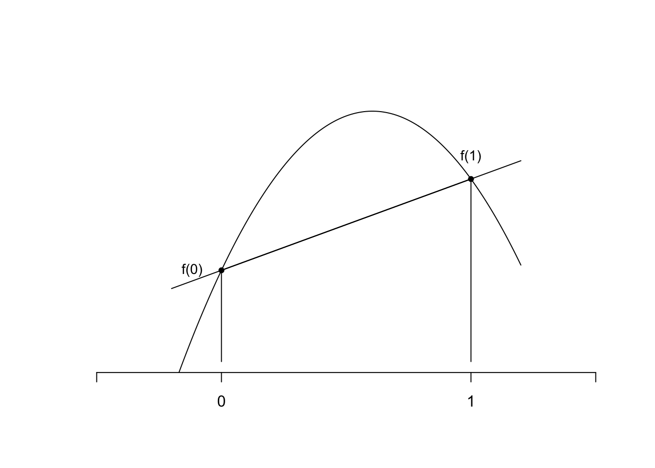
Figure 3.1: The trapezium rule

For \(N=2\), we have three points \(x_0=0\), \(x_1=1\), and \(x_2=1/2\). Using the Newton divided-difference form of the quadratic interpolant, \[\begin{equation*} p_2(x) = f(0)+f[0,1]x+ f[0,1,1/2]x(x-1). \end{equation*}\] Then, \[\begin{align*} \int^1_0 p_2(x)\,dx & = f(0) + \frac12 f[0,1] +f[0,1,1/2] \underbrace{\int^1_0 (x^2-x)\,dx}_{= -1/6}\\ &= f(0) + \frac12 \frac{f(1)-f(0)}1 - \frac16 \frac{f[0,1/2]-f[0,1]}{1/2-1}, \end{align*}\] where \(f[0,1/2]=2(f(1/2)-f(0))\) and \(f[0,1]=f(1)-f(0)\). Thus, \[\begin{align*} \int^1_0 p_2(x)\,dx &= f(0) + \frac12 (f(1)-f(0)) +\frac13 \left({ 2f(1/2)-2f(0)+f(0)-f(1)}\right)\\ &= \frac16\left[{f(0)+4f\left({\textstyle \frac12}\right)+f(1)}\right]. \end{align*}\] This is called Simpson’s rule. We write \[\begin{equation} \tag{3.4} Q_2(f) \colon= \frac16f(0)+ \frac46 f\left({\textstyle \frac12}\right)+ \frac16f(1), \end{equation}\] with weights \(w_0 = w_1 = \frac{1}{6}\) and \(w_2 = \frac{4}{6}\). This rule is exact for all \(f \in \mathcal{P}_2\), since again in that case \(p_2 = f\).

In general, Newton–Cotes quadrature rules are of the form \[ Q_N(f) \colon= \sum^N_{i=0}w_if(x_i) \] where \(x_i= i/N\) for \(i=0,\dots,N\), and the weights \(w_i\) can be found by integrating the degree-\(N\) interpolating polynomial. By writing \(p_N(x)\) using the Lagrange basis functions (see the proof of Theorem 2.2), \[ p_N(x)=\sum_{i=0}^N L_i(x) f(x_i), \] we can show that \[ w_i=\int_0^1 L_i(x)\,dx. \]

3.1.2 Newton–Cotes rules over a general interval \([a,b]\)

Suppose now we have a rule \[\begin{equation} \tag{3.5} Q(f) = \sum_{i=0}^N w_i f(x_i)\quad \quad \text{that approximates} \quad \quad \int_0^1 f(x) \,dx. \end{equation}\] To approximate $_a^b f(t), dt $, we make a change of variable \(\displaystyle x = \frac{t-a}{b-a}\) and \(dx=\frac{1}{b-a}dt\). Then, \(t \in [a,b]\) is mapped to \(x\in [0,1]\) and \[ \int^b_a f(t) \,dt =\int^1_0 \underbrace{(b-a)f\left({a+x(b-a)}\right)}_{\textstyle =\colon g(x)}\,dx = \int_0^1 g(x) \,dx. \]

We now use \(Q(g)\) to approximate the right-hand side, to obtain the rule \[\begin{equation} Q^{[a,b]}(f) \colon= \sum_{i=0}^N w_i g(x_i) = (b-a) \sum_{i=0}^N w_i f\left({a + (b-a) x_i}\right). \tag{3.6} \end{equation}\]

Notation: We use superscript \([a,b]\) to denote a rule over \([a,b]\). We omit the superscript for \([0,1]\). The lowest-order Newton–Cotes rules on a general interval \([a,b]\) are \[\begin{alignat*}{2} Q_{1}^{[a,b]}(f) & = \frac{b-a}{2} \left({f(a) + f(b)}\right), &\text{trapezium rule}\\ Q_{2}^{[a,b]}(f) & = \frac{b-a}{6} \left({f(a) + 4 f\left({\frac{b + a}{2}}\right) + f(b)}\right), \qquad &\text{Simpson's rule.} \end{alignat*}\]

Example 3.1 Let us apply these to the integral of \(f(x) = \sqrt{x}\) over \([1/4,1]\). Then \[ Q_1^{[1/4,1]} (f) = \frac{1 - \frac{1}{4}}{2} \left({\sqrt{1/4} + 1}\right) = \frac{3}{8} \, \frac{3}{2} = 9/16 = 0.5625, \qquad\quad \text{trapezoidal} \] \[ Q_2^{[1/4,1]} (f) = \frac{1 - \frac{1}{4}}{6} \left({\sqrt{1/4} + 4 \sqrt{5/8} + 1}\right) =0.582785\quad\text{(6 s.f.),} \quad \text{Simpson's.} \] The exact value \[ \int^1_{1/4}\sqrt{x}\,dx = \frac{2}{3} \left[{x^{3/2}}\right]_{1/4}^1 = \frac{7}{12} = 0.583333\quad \text{(6 s.f.)}, \] so the absolute value of the error in Simpson’s rule is \(\lvert{ 0.582785 - 0.583333 }\rvert = 5.48 \times 10^{-4}\), which is about 38 times smaller than the error in the trapezoidal rule \(\lvert{ 9/16 - 0.583333 }\rvert = 2.083\times 10^{-2}\).

3.1.3 Composite rules

As for the piecewise interpolation in 2, instead of increasing the accuracy of quadrature by choosing higher-order interpolating polynomials, we can also split the integration domain into subintervals by introducing a mesh and applying low-order rules on the sub-intervals.

Consider a general quadrature rule (e.g., from Section 3.1 \[\begin{equation} \tag{3.7} Q(f) = \sum_{i=0}^N w_if(x_i) \quad \text{that approximates} \quad \int^1_0f(x)\,dx, \end{equation}\] for some \(N\), weights \(w_i\) and distinct points \(x_i\). To approximate \(\int_a^b f(t)\, dt\), we introduce the mesh \(a = y_0 < y_1 < \cdots < y_J = b\) and write \[ \int_a^b f(t)\, dt = \int_{y_{0}}^{y_1} f(t) \, dt + \int_{y_{1}}^{y_2} f(t) \, dt + \cdots + \int_{y_{J-1}}^{y_J} f(t) \, dt = \sum_{j=1}^J \int_{y_{j-1}}^{y_j} f(t) \, dt. \] Now use the quadrature rule given by (3.7) on each subinterval, to obtain the approximation \[\begin{equation} \int_a^b f(t) \,dt \approx \sum_{j=1}^J Q^{[y_{j-1}, y_j]} (f) = \sum_{j=1}^J h_j \sum_{i=0}^N w_i f(y_{j-1}+h_jx_i), \tag{3.8} \end{equation}\] where \(h_j = y_j - y_{j-1}\). The approximation (3.8) is known as the composite version of (3.7).

As in the case of interpolation, we expect that accuracy will increase when the mesh width \(\max_j h_j \rightarrow 0\).

Example 3.2 (composite trapezoidal rule)

\[\begin{equation} \tag{3.9} Q_{1,J}^{[a,b]}(f) \colon= \sum_{j = 1}^J Q_1^{[y_{j-1},y_j]}(f) = \sum_{j=1}^J\frac{h_j}{2}\left({f(y_{j-1})+f(y_j)}\right). \end{equation}\] For a uniform mesh, \(h_j = h \colon= (b-a)/J\),, \(j=1,\ldots,J\), this can be written compactly as \[ Q_{1,J}^{[a,b]}(f) \colon= h \left({ \frac{f(a)}{2} + \sum_{j=1}^{J-1} f(y_j) \; + \; \frac{f(b)}{2} }\right). \]

Example 3.3 (composite Simpson’s rule)

\[\begin{equation} \tag{3.10} Q_{2,J}^{[a,b]}(f) \colon= \sum_{j=1}^J Q_2^{[y_{j-1}, y_j]}(f) = \sum_{j=1}^J\frac{h_j}{6}\left({f(y_{j-1})+4f(m_j) + f(y_j)}\right), \end{equation}\] where the midpoints \(\displaystyle m_j = \frac{y_{j-1} + y_j}{2}\). For a uniform mesh, this can again be written more compactly as \[ Q_{2,J}^{[a,b]}(f) =\frac{h}{6}\left[{ f(a) + 2 \sum_{j=1}^{J-1}f(y_j) + 4 \sum_{j=1}^{J} f(m_j) + f(b) }\right]. \]

Please implement the general formulae (3.9) and (3.10) in Python, so that we can apply the rules on any mesh.

3.2 Error analysis

3.2.1 Non-composite rules over \([0,1]\)

Given a rule \[\begin{equation} \tag{3.11} Q(f) \colon= \sum_{i=0}^N w_if(x_i) \end{equation}\] that approximates \[I(f) \colon= \int^1_0f(x)\,dx,\] we define the error in the quadrature rule to be \[\begin{equation} \tag{3.12} E(f) \colon= I(f) - Q(f) \; . \end{equation}\]

Definition 3.1 (DoP) The rule \(Q(f)\) in (3.11) has degree of precision (DoP) \(d\in\mathbb{N}\) if

\[ E(x^r)=0 \quad \text{ for all $r\in\mathbb{N}$ with $0\le r \leq d, \qquad$ and $E(x^{d+1}) \ne 0$.} \]

Example 3.4 (trapezium rule DoP) The trapezium rule \(Q_1(f)=\frac12(f(0)+f(1))\), and the error \(E_1(f) \colon= I(f)-Q_1(f)\). We create the following table:

\(r\)	\(x^r\)	\(I(x^r)\)	\(Q_1(x^r)\)	\(E_1(x^r)\)
0	1	1	\(\frac12\cdot 1 + \frac12\cdot 1 = 1\)	0
1	\(x\)	\(\frac12\)	\(\frac12\cdot 0 + \frac12\cdot 1 = \frac12\)	0
2	\(x^2\)	\(\frac13\)	\(\frac12\cdot 0 + \frac12\cdot 1 = \frac12\)	\(-\frac16\)

Hence the DoP of the trapezoidal rule is \(1\).

Example 3.5 (Simpson’s rule DoP) Simpson’s rule \(Q_2(f)=\frac16 \left[ {f(0)+4f\left(\frac12\right)+f(1)} \right]\), and the error \(E_2(f) \colon= I(f)-Q_2(f)\). We create the following table:

\(r\)	\(x^r\)	\(I(x^r)\)	\(Q_2(x^r)\)	\(E_2(x^r)\)
0	1	1	\(\frac16\left(1\cdot 1 + 4\cdot 1 + 1\cdot 1\right) = 1\)	0
1	\(x\)	\(\frac12\)	\(\frac16\left(1\cdot 1 + 4\cdot \frac12 + 1\cdot 1\right) = \frac12\)	0
2	\(x^2\)	\(\frac13\)	\(\frac16\left(1\cdot 1 + 4\cdot \left(\frac12\right)^2 + 1\cdot 1\right)= \frac13\)	0
3	\(x^3\)	\(\frac14\)	\(\frac16\left(1\cdot 1 + 4\cdot \left(\frac12\right)^3 + 1\cdot 1\right)= \frac14\)	0
4	\(x^4\)	\(\frac15\)	\(\frac16\left(1\cdot 1 + 4\cdot \left(\frac12\right)^4 + 1\cdot 1\right)= \frac{5}{24}\)	\(-\frac{1}{120}\)

Hence the DoP of Simpson’s rule is \(3\).

The trapezium rule \(Q_1\) is found by integrating \(p_1\) and it is not surprising that its DoP is 1. Similarly, \(Q_2\) is found by integrating \(p_2\) and thus we’d expect a DoP of at least 2. A DoP of \(3\) is a surprise.
In fact, it turns out that for all \(N \in \mathbb{N}\) the Newton–Cotes rule \(Q_N(f)\) is of DoP \(N\) if \(N\) is odd and of DoP \(N+1\) if \(N\) is even.

Proposition 3.1 If (3.11) has DoP \(d\), then \[ E(p) = 0,\quad \text{for all} \quad p\in \mathcal{P}_d. \]

Proof. For any \(f_1, f_2\colon [0,1]\to \mathbb{R}\) and \(\alpha,\beta\in\mathbb{R}\), \[\begin{equation} I(\alpha f_1+\beta f_2)\; =\; \alpha I(f_2)+\beta I(f_2)\quad\text{and}\quad Q(\alpha f_1+\beta f_2) \; = \; \alpha Q(f_2)+\beta Q(f_2), \tag{3.13} \end{equation}\] since \(I\) and \(Q\) are both linear transformations.

If \(p\in\mathcal{P}_d\), \(p\) is a polynomial of degree less than or equal to \(d\) and can be written \[ p(x)=\sum^d_{r=0}a_rx^r,\quad\text{for some coefficients } a_r \in \mathbb{R}. \] Hence, using (3.13), \[ I(p)-Q(p) = \sum^d_{r=0} a_r \left[{I(x^r)-Q(x^r) }\right] = 0, \] since the DoP equals \(d\).

With significant further work, we can show that, for the trapezium rule, there exists \(\xi\in[0,1]\) such that \[\begin{equation} \tag{3.14} E_1(f) = \left[{ \frac{E_1(x^2)}{2!}}\right] f''(\xi) = - \frac{1}{12} f''(\xi), \qquad \text{for all} \ f \in C^2[0,1]. \end{equation}\] For \(p\in \mathcal{P}_1\), \(p''\equiv 0\) and \(E_1(p)=0\) as expected from the DoP calculation.

For Simpson’s rule, there exists \(\xi\in[0,1]\) such that \[ E_2(f)= \left[{\frac{E_2(x^4)}{4!}}\right]f^{(\mathrm{4})}(\xi) = - \frac{1}{2880} f^{(\mathrm{4})}(\xi), \qquad \text{for all} \ f \in C^4[0,1]. \] Notice the error for Simpson’s rule depends on the fourth derivative of \(f\) while that for the trapezium rule depends on the second derivative. Here \(C^k[a,b]\) is the set of functions \(f\colon [a,b]\to \mathbb{R}\) that are \(k\)-times continuously differentiable.

This leads to estimates over \([a,b]\) instead of \([0,1]\) by a change of variables.

Example 3.6 The error for the trapezoidal rule over \([a,b]\) is \[ E_1^{[a,b]} (f) \colon= \int_a^b f(t)\, dt - Q_1^{[a,b]}(f). \] To determine the error, we recall that \[ \int_a^b f(t) \,dt =\int_0^1 g(x)\,dx,\qquad Q_1^{[a,b]}(f)=Q_1(g), \] from (3.6) with \(g(x)=(b-a) f(a+(b-a)x)\). Now \(g'(x)=(b-a)^2 f'(a+(b-a)x)\) and \(g''(x)=(b-a)^3 f''(a+(b-a)x)\). By (3.14), \[ E_1(g) = \int_0^1 g(x)\,dx - Q_1(g)=-\frac{1}{12}g''(\xi)=-\frac{1}{12} (b-a)^3 f''(\eta) \] for some \(\xi\in[0,1]\) and \(\eta\colon= a+(b-a)\xi\). Then, \[ E_1^{[a,b]} (f) = - \frac{(b-a)^3}{12} f''(\eta) \quad \quad \text{ for some} \quad \eta \in [a,b]. \] A similar calculation shows that the error for Simpson’s rule over \([a,b]\) is \[ E_2^{[a,b]} (f) \colon= \int_a^b f (t) \,dt - Q_2^{[a,b]}(f) = - \frac{(b-a)^5}{2880} f^{(4)}(\eta) \qquad \text{ for some $\eta \in [a,b]$.} \] Notice the fifth power of \((b-a)\), which comes from the change of coordinates from \(t\) to \(x\).

3.2.2 Composite Newton–Cotes rules

Let \(Q_N\) be a Newton–Cotes rule on \([0,1]\) with degree of precision \(d\). The composite version with \(J\) subintervals on \([a,b]\) is (as in Section 3.1.3): \[ Q_{N,J}^{[a,b]}(f) = \sum_{j=1}^J Q_N^{[y_{j-1},y_j]}(f). % \] The error can be expressed in terms of the error made in approximating the sub-integrals. \[ E_{N,J}^{[a,b]}(f) \colon= \int_a^b f(x) \,dx - Q_{N,J}^{[a,b]}(f) = \sum_{j=1}^J \underbrace{\left[{ \int_{y_{j-1}}^{y_j} f(x)\,dx - Q_N^{[y_{j-1},y_j]}(f)}\right]}_{=E_N^{[y_{j-1},y_j]}(f)}. \] We have formula for \(E_N^{[a,b]}\) for \(N=1,2\), which lead to the following error estimates for the composite trapezium and Simpson’s rule.

Example 3.7 (Composite trapezium rule error) If \(f \in C^2[a,b]\), then there exists \(\eta_j \in [y_{j-1},y_j]\) such that \[ E_{1,J}^{[a,b]} (f) = - \frac{1}{12} \sum_{j=1}^J h^{3}_j f^{(2)}(\eta_j) \qquad \text{and} \qquad \lvert{E_{1,J}^{[a,b]}\rvert (f)} \le \frac{b-a}{12} \lVert{ f^{(2)} }\rVert_{\infty,[a,b]} h^2, \] since \(\sum_{j=1}^J h_j=b-a\).

Example 3.8 (Composite Simpson’s rule error) If \(f \in C^4[a,b]\), then there exists \(\eta_j \in [y_{j-1},y_j]\) such that \[ E_{2,J}^{[a,b]} (f) = - \frac{1}{2880} \sum_{j=1}^J h^{5}_j f^{(4)}(\eta_j) \qquad \text{and} \qquad \lvert{E_{2,J}^{[a,b]} (f)}\rvert \le \frac{b-a}{2880} \lVert{ f^{(4)} }\rVert_{\infty,[a,b]} h^4. \]

If \(f(x)\) fails to be sufficiently differentiable on all of \([a,b]\), but is sufficiently differentiable on subintervals of \([a,b]\), we can apply error estimates there.

Example 3.9 Consider \(f(x) = \sqrt{x}\) on \([0,1]\), which has infinitely many derivatives on subintervals that do not contain~\(0\), but no bounded derivatives on \([0,1]\). Consider the composite trapezoidal rule for \(\int_0^1 f(x) \,dx\) on the mesh \(0=y_0 < y_1 < \cdots < y_J=1\). Then \[\begin{align} E_{1,J}^{[0,1]} (f) = & E_{1,J}^{[0,y_1]} (f) + E_{1,J}^{[y_1,1]} (f) \nonumber \\ = & \left({ \int_0^{y_1} f(x) \, \,dx - h_1 \frac{\sqrt{y_1}}{2} }\right) - \frac{1}{12} \sum_{j=2}^J h_j^{3} f^{(2)}(\eta_j)\;. \tag{3.15} \end{align}\] Now, we can estimate each of the terms in (3.15) separately (see Problem E5.2).

3.3 Gaussian quadrature rules

The only examples of quadrature rules so far have been Newton–Cotes rules with equally spaced points. Can we do better with other points?

To take advantage of symmetry and simplify calculations, we work on the interval \([-1,1]\) rather than \([0,1]\) (which can of course be transformed onto \([0,1]\)). Let \(x_i\), \(i=0,\dots,N\), be in \([-1,1]\), and let \(p_N(x)\) be the degree-\(N\) interpolating polynomial for a function \(f\) at these points. Consider the rule:

\[\begin{equation} \tag{3.16} Q_{\mathrm{Gauss},N}^{[-1,1]}(f)\colon= \int^1_{-1}p_N(x)\,dx \end{equation}\] as an approximation to \[\begin{equation} \tag{3.17} \int^1_{-1}f(x)\,dx. \end{equation}\] This rule has DoP at least \(N\). Can we do better with a clever choice of points? There are \(2N+2\) degrees of freedom (given by choice of \(x_i\) and \(w_i\) for \(i=0,\dots,N\)) and \(d+1\) conditions to achieve of a DoP of \(d\). By equating the number of conditions to the number of degrees of freedom, \(d+1=2N+2\), we hope that a DoP \(d=2N+1\) can be achieved by careful choice of \(x_i\) and weights \(w_i\).

Example 3.10 (One point, \(N=0\)) To achieve a DoP of \(d=2N+1=1\), we demand that \[\begin{equation} \tag{3.18} Q(1) = \int_{-1}^1 1\,dx=2\qquad\text{and}\qquad Q(x) =\int_{-1}^1 x\,dx=0. \end{equation}\] As \(p_0(x)\) is a constant, we must have \(p_0(x)=f(x_0)\) and \[ Q(f)=w_0 f(x_0). \] Then, \(w_0=2\) and \(x_0=0\) gives (3.18). Therefore, the one-point Gauss rule (or midpoint rule), obtained by integrating the degree-0 interpolant \(p_0\) at \(x_0=0\) over \([-1,1]\) is \[\begin{align*} Q_{\mathrm{Gauss},0}^{[-1,1]}(f) \colon= \int^1_{-1} p_0(x)\,dx = 2 f(0). \end{align*}\] This is exact when \(f=1\) and \(f=x\), so it is a one-point rule with DoP \(=1\). Any other one-point rule has only DoP \(=0\).

Example 3.11 (Two points, \(N=1\)) To achieve a DoP \(d=2N+1=3\), we demand that \[ Q(1)=2,\qquad Q(x)=0, \qquad Q(x^2)=\frac{2}{3},\qquad\text{and}\qquad Q(x^3)=0. \] As \[ Q(f)= w_0 f(x_0)+w_1 f(x_1), \] we must have \(w_0+w_1=2\) and \(w_0 x_0 +w_1 x_1=0\) and \(w_0 x_0^2+w_1 x_1^2=2/3\) and \(w_0 x_0^3+ w_1 x_0^3=0\). By symmetry considerations, we must have \(x_0=-x_1\) and \(w_0=w_1\). Then \(w_0=w_1=1\) and \(2 x_0^2=2/3\), so that \(x_0=\sqrt{1/3}\). We obtain the two-point Gauss rule \[\begin{align*} Q_{\mathrm{Gauss},1}^{[-1,1]}(f) \colon= \int^1_{-1} p_1(x)\,dx = f\left({\frac{1}{\sqrt3}}\right) + f\left({-\frac{1}{\sqrt3}}\right). \end{align*}\] Although only a two-point rule, its DoP is \(2N +1 = 3\). Compare with the trapezium rule which uses two points and has DoP only \(1\)!

Remark. Composite Gauss rules can also be derived and are highly effective.

High-frequency integrands, where \(f\) oscillates rapidly and where the derivatives of \(f\) are large, are particularly difficult and arise, for example, in high-frequency scattering applications (e.g., radio waves). This requires special techniques such as Filon quadrature.

Multivariate integrals are also important. For low-dimensional problems, simple (applying one-dimensional rules in each dimension) work fine and our theory carries over easily. For high-dimensional integrals, the only feasible methods currently are .