Chapter 2 Interpolation

Problem Suppose that a function \(f\colon [a,b]\to\mathbb{R}\) is specified only by its values \(f(x_i)\) at the \(N+1\) distinct points \(x_0,x_1,\dots,x_N\). How can we approximate \(f(x)\) for all \(x\)?

In polynomial interpolation, we do this by constructing a polynomial \(p_N\) of degree \(N\) such that

\[\begin{equation} p_N(x_i)=f(x_i), \qquad i = 0, \ldots , N . \tag{2.1} \end{equation}\]

2.1 Linear interpolation

Linear interpolation is the case \(N=1\). We are given two points \(x_0 \neq x_1\) and values \(f(x_0)\) and \(f(x_1)\). The interpolant \(p_1(x)\) is simply the straight line given by \[\begin{equation} \tag{2.2} p_1(x) =f(x_0)+\left(\frac{f(x_1)-f(x_0)}{x_1-x_0}\right)(x-x_0). \end{equation}\]

You should check that \(p_1\) is linear and \(p_1(x_i) = f(x_i)\) for \(i = 0,1\).

Example 2.1 Approximate \(f(x)=\sqrt{x}\) by linear interpolation at \(x_0=1/4\) and \(x_1=1\).

By (2.2), \[\begin{align*} p_1(x)& = \sqrt{\frac14} + \left(\frac{1-\sqrt{\frac14}}{1-\frac14}\right)(x-\frac14) \\ &= \frac{2}{3}x+ \frac{1}{3}. \end{align*}\]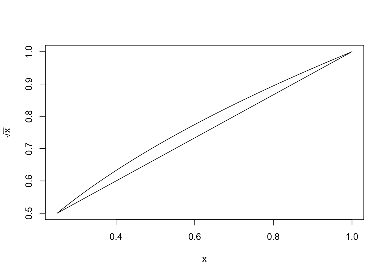

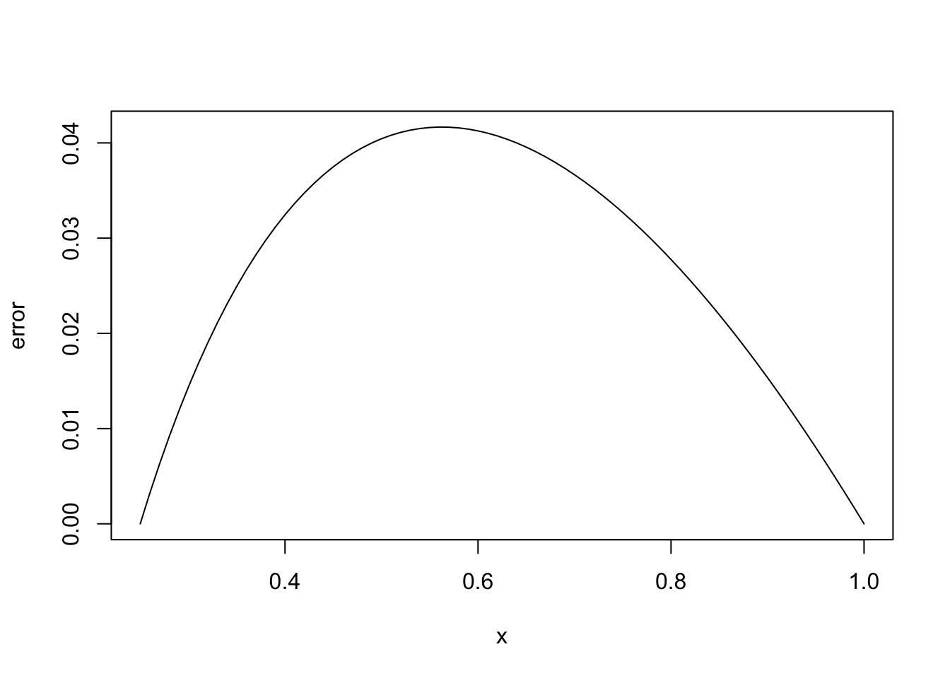
Figure 2.1: Linear interpolation of \(f(x) = \sqrt{x}\) at \(x_0 = 1/4\) and \(x_1 = 1\)

Figure 2.1 shows graphs of \(f(x)\) and \(p_1(x)\) for \(x_0 = 1/4\) and $ x_1 =1$, and the error at each point.

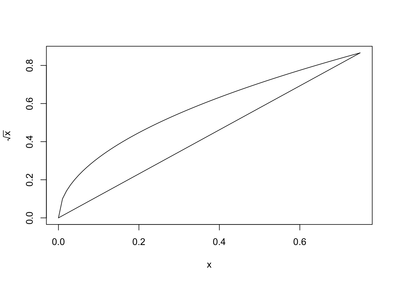
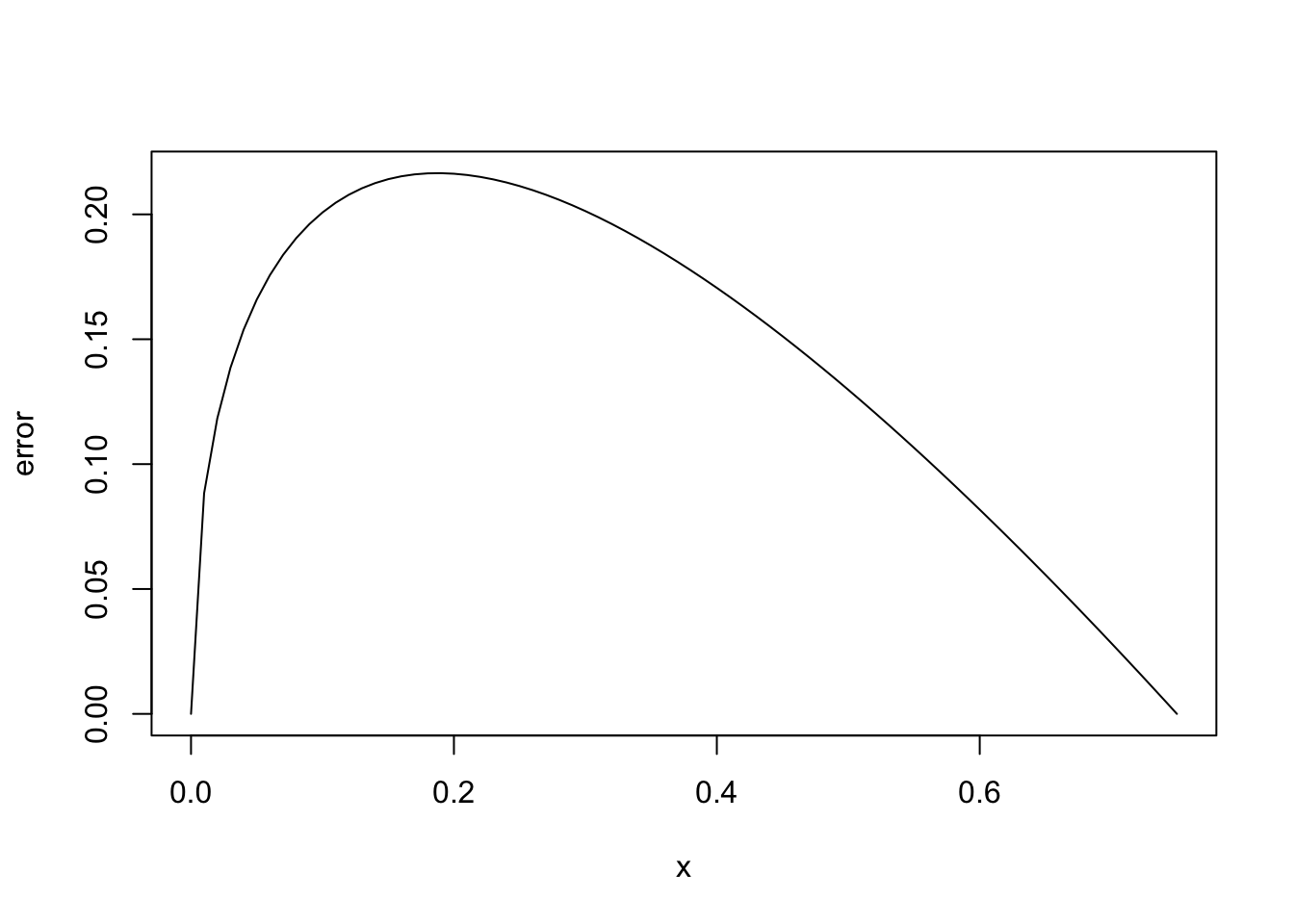
Figure 2.2: Linear interpolation of \(f(x) = \sqrt{x}\) at \(x_0 = 0\) and \(x_1 = 3/4\)

Figure 2.2 shows the same graphs for \(x_0 = 0\) and \(x_1 =3/4\).The error in the second example is much bigger! Let us explain why.

Corollary 2.1 (Rolle’s theorem) Let \(f\colon [a,b]\to \mathbb{R}\) be smooth with \(f(a) = f(b)\). There exists \(\xi \in (a,b)\) such that \(f'(\xi) = 0\).

Proof. This is a special case of the mean-value theorem using \(f(a)=f(b)\).

To analyse the error in linear interpolation, set \[\begin{align*} e(x) \colon= f(x)-p_1(x). \end{align*}\] Note that \(e(x_0) = 0 = e(x_1)\).

Theorem 2.1 Suppose that \(f\colon [x_0,x_1]\to \mathbb{R}\) is smooth. For all \(x\in(x_0,x_1)\), there exists \(\xi\in(x_0,x_1)\) such that

\[\begin{equation} \tag{2.3} e(x)=\frac{f''(\xi)}{2}w_2(x),\quad\text{where}\quad w_2(x) \colon= (x-x_0)(x-x_1). \end{equation}\]

Proof. Fix \(x\in(x_0,x_1)\) and note that \(w_2(x) \ne 0\). Define \[\begin{equation} \tag{2.4} g(t) \colon= e(t)-\frac{e(x)}{w_2(x)}w_2(t)\qquad \text{for $t\in[x_0,x_1]$.} \end{equation}\]

Observe that \[ g(x_0) =e(x_0)-\frac{e(x)}{w_2(x)}w_2(x_0)=0-0=0. \] Similarly \(g(x_1)=0\).

Also, \[ g(x) =e(x)-\frac{e(x)}{w_2(x)}w_2(x) = e(x) - e(x) = 0 . \]

The smoothness assumption of \(f\) implies smoothness of \(g\) and Rolle’s theorem applies. Hence, applying Rolle’s theorem twice, \[ \exists \eta_1\in(x_0,x), \eta_2\in(x,x_1) \quad \text{ such that $g'(\eta_1)=0=g'(\eta_2)$.} \] Now consider \(g'(t)\): \[ g'(t) = e'(t) - \frac{e(x)}{w_2(x)} w_2'(t). \] Hence, Rolle’s theorem implies again and \[\begin{equation} \tag{2.5} \exists \xi\in(\eta_1,\eta_2) \quad \text{ such that $g''(\xi)=0$.} \end{equation}\]

By (2.4), \[ g(t) =f(t)-p_1(t)-\frac{e(x)}{w_2(x)}(t-x_0)(t-x_1). \] Since \(p_1\) is a linear function, \(p_1''(t) \equiv 0\) and so \[ g''(t) =f''(t)-0-2 \frac{e(x)}{w_2(x)}. \] As \(g''(\xi)=0\) by (2.5), \[ 0 = f''(\xi) - 2\frac{e(x)}{w_2(x)}\] and finally this can be rearranged to show that (2.3) holds.

We note that \(\xi\) in (2.3) depends on \(x\) and we do not know it explicitly in general. We only know that it exists. This makes the above formula for the error difficult to use. To get around this, we replace the term involving \(\xi\) by something that is easier to understand.

Definition 2.1 For any interval \(I\) and \(f\colon I \to \mathbb{R}\), we define the sup norm \[ \lVert{f}\rVert _{\infty, I} \colon= \sup_{x \in I} \lvert{ f(x) }\rvert. \]

Here, \(\sup\) means supremum or least upper bound and, in many cases, it is the same as finding the maximum of \(\lvert{ f(x) }\rvert\) on \(I\).

Corollary 2.2 Under the assumptions of Theorem 2.1, \[\begin{equation} \tag{2.6} \lVert{e}\rVert_{\infty,[x_0,x_1]} \leq \frac{(x_1-x_0)^2}{8}\lVert{ f''}\rVert_{\infty,[x_0,x_1]}. \end{equation}\]

Proof. From Theorem 2.1, for all \(x \in (x_0,x_1)\), \[ \lvert{e(x)}\rvert = \frac{\lvert f''(\xi)\rvert}{2}\lvert w_2(x) \rvert,\quad \text{for some $\xi\in(x_0,x_1)$.} \] Also, \[ \lvert {w_2(x)} \rvert = \lvert(x-x_0)(x-x_1)\rvert = (x-x_0)(x_1-x). \] Simple calculus (see Problem E2.1) shows that \[ \lvert {w_2(x)} \rvert \le \frac{(x_1-x_0)^2}{4}. \] Hence, \[ \lvert {e(x)} \rvert \leq \frac{(x_1 - x_0)^2}{8} \lVert{ f'' }\rVert_{\infty, [x_0,x_1]}. \] This inequality also holds for \(x = x_0\) and \(x_1\) (since the left-hand side vanishes) and we have derived (2.6).

The smoothness of \(f\) affects the quality of the approximation and we see that the error is proportional to \(f''(\xi)\). The size of the derivatives of \(f\) is one way to quantify the smoothness of a function. In Figure 2.1, \(f(x)=\sqrt{x}\) on \([1/4,1]\) and in Figure 2.2 the interval is \([0,3/4]\). Because \(f''(x)\to\infty\) as \(x \to 0\), \(\lVert{f''}\rVert_{\infty,[0,3/4]}\) is infinite and the error is much larger in the second example.

See Problem E2.4 for a computational example.

2.1.1 Piecewise-linear interpolation

To get a (more) accurate approximation to \(f \colon [a,b] \rightarrow \mathbb{R}\), we subdivide \([a,b]\) into a of points \[ a = y_0 < y_1 < \dots < y_J = b \] and use linear interpolation on each subinterval \([y_{j-1}, y_j]\).

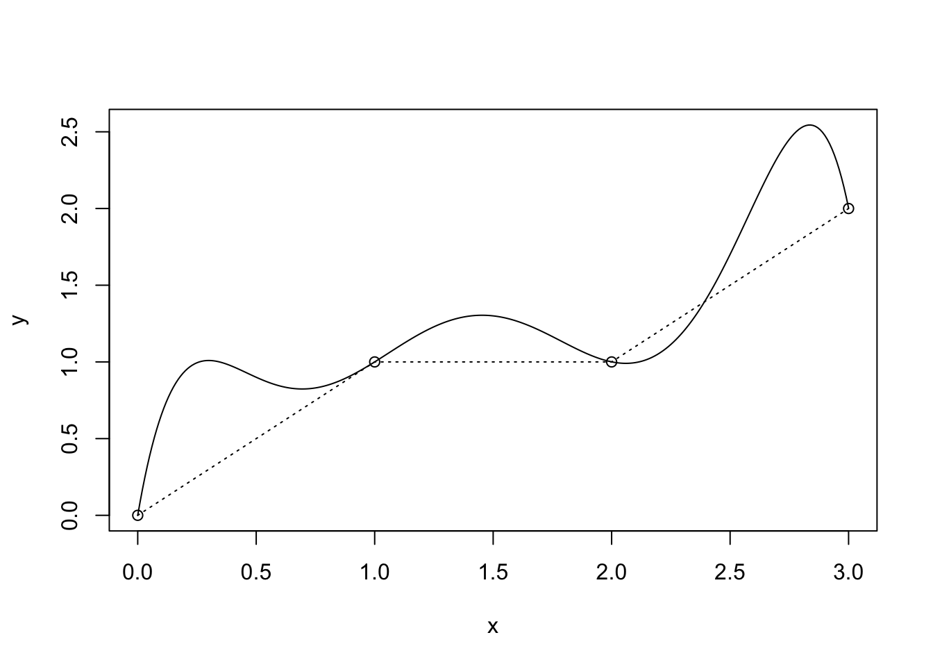
Figure 2.3: Piecewise-linear interpolation

Let \(p_{1,J}\) denote the on \([a,b]\) that interpolates \(f\) at all the points \(y_j\) of the mesh and let \(h_j \colon= y_j - y_{j-1}\). By Corollary 2.2, \[ \lVert{ f-p_{1,J}}\rVert_{\infty,[y_{j-1},y_j]} \le \frac{1}{8} h_j^2 \lVert{ f''}\rVert_{\infty, [y_{j-1}, y_j]}. \] Clearly, \[ \lVert{ f-p_{1,J}}\rVert_{\infty,[a,b]} =\max_{j=1,\dots,J} \lVert{ f-p_{1,J}}\rVert_{\infty,[y_{j-1},y_j]}. \] Hence, in terms of the mesh width \(h \colon= \max_{j=1,\dots,J} h_j\), \[\begin{equation} \tag{2.7} \lVert{ f-p_{1,J}}\rVert_{\infty,[a,b]} \le \frac{1}{8} h^2 \max_{j=1,\dots,J} \lVert{ f''}\rVert_{\infty, [y_{j-1}, y_j]} = \frac{1}{8} h^2 \lVert{ f''}\rVert_{\infty, [a,b]}. \end{equation}\] Convergence is achieved as \(h \rightarrow 0\) and the error is \(\mathcal{O}({h^2})\).

At the points \(y_j\), the function \(f\) is only required to be continuous! It does not need to be twice continuously differentiable at \(y_j\). If all discontinuities in \(f'\) are resolved by the mesh, we can deal with less smooth functions in piecewise interpolation.

Example 2.2 Let \(f(x) = \exp(x^2)\) on \([a,b] = [0,1]\) and let \(y_j = j h, j = 0, \ldots , J\), where \(h = 1/J\) (this is called a uniform mesh). In Problem E3.1, you will write a program to compute \[ e_h \colon= \max_{j = 1, \ldots , J} \lvert{ (f - p_{1,J})(z_j)}\rvert \] where \(z_j \colon= (y_{j-1} + y_j)/2\) (the midpoint of \([y_{j-1}, y_j]\)). A discrete set of points is used for the maximum instead of the whole interval, to allow easy computation.

\(h\)	\(e_h\)	\((e_h)/(e_{h/2})\)	bound\((h)\)
1/8	2.60e-2	3.62	3.18e-2
1/16	7.19e-3	3.80	7.95e-3
1/32	1.89e-3	3.90	1.99e-3
1/64	4.85e-4		4.97e-4

To estimate the rate of convergence, we conjecture that \(e_h = C h^\alpha\). Then, \[ (e_h)/(e_{h/2}) = 2^{\alpha}. \] The third column suggests \(\alpha\) approaches \(2\). To prove this rigorously, note that \[ f''(x) = (4x^2 + 2) \exp(x^2) \qquad \Rightarrow \qquad \lVert{ f''}\rVert_{\infty,[0,1]} \leq 6 \exp(1). \] Hence, from (2.7), \[ e_h \le \lVert{ f - p_{1,J}}\rVert_{\infty, [0,1]} \le \frac{1}{8} h^2 \lVert{ f''}\rVert_{\infty,[0,1]} \le \frac{3}{4} \exp(1) h^2 =\colon \mathrm{bound}(h). \] Note how sharp the theoretical bound is (in the table)!

2.2 Degree-\(N\) interpolation

When \(f\) is smooth, better accuracy is possible by choosing the degree-\(N\) polynomial that interpolates at \(N+1\) distinct points instead. Let \(\mathcal{P}_N\) denote the polynomials of degree \(N\) or less.

Problem Given \(N+1\) distinct points \(x_0,\dots,x_N\) and values \(f(x_0),\dots,f(x_N)\), compute a polynomial \(p_N\in\mathcal{P}_N\) with the property that \[\begin{equation} \tag{2.8} p_N(x_i) =f(x_i),\qquad i=0,\dots,N. \end{equation}\]

We finish this chapter with two theorems:

Theorem 2.2 (Existence and Uniqueness) Let \(x_0, x_1 , \cdots , x_N\) be distinct points in \([a,b]\) and suppose \(f\colon [a,b] \to \mathbb{R}\) is continuous. Then, there exists a unique \(p_N \in \mathcal{P}_N\) satisfying \(p_N(x_i) = f(x_i)\) for \(i = 0, \ldots , N\).

Proof. Let \[ L_j(x) \colon= \frac{\prod_{i\ne j}(x-x_i)}{\prod_{i\ne j}(x_j-x_i)}, \] where \(\prod\) denotes the product of each term. These are known as {Lagrange basis functions} and are degree-\(N\) polynomials (i.e., \(L_j\in \mathcal{P}_N\)). Note that \(L_j(x_k)=\delta_{jk}\) (the Kronecker delta function), with \(\delta_{jk}=0\) if \(j\ne k\) and \(\delta_{jk}=1\) if \(j=k\). Define \[ p_N(x) =\sum_{j=0}^N f(x_j) L_j(x). \] Then, evaluating at \(x=x_i\), we have \[ p_N(x_i) =\sum_{j=0}^N f(x_j) \delta_{ij}=f(x_i). \] This is a degree-\(N\) interpolant of \(f\) and we have proved existence.

To show uniqueness, let \(p,q \in \mathcal{P}_N\) both satisfy (2.8). Then \(p,q\) agree at \(N+1\) distinct points and \(r\colon= p-q\) is a degree-\(N\) polynomial with \(N+1\) distinct roots. This can only happen if \(r\equiv 0\) and the polynomials \(p\) and \(q\) are identical.

The following theorem generalises Theorem 2.1 to general \(N\). We assume the points are well ordered so that \(x_i<x_{i+1}\).

Theorem 2.3 Suppose the conditions of Theorem 2.1 hold and that \(f\) is smooth. Then, for all \(x\in[x_0,x_N]\), there exists \(\xi \in (x_0,x_N)\) such that \[ (f - p_N)(x) =\frac{f^{(N+1)}(\xi)}{(N+1)!}w_{N+1}(x). \] where \(w_{N+1}(x)=(x-x_0)\times \dots\times (x-x_{N})\).

Proof. Not covered.

Notice that now derivatives of order \(N+1\) determine the quality of the approximation. It is easy to show that \(w_{N+1}(x)=\mathcal{O}({h^{N+1}})\) if \(\lvert x-x_j \rvert \le h\). Hence, if \(f\) is \((N+1)\)-times continuously differentiable, \(\lVert{f-p_N}\rVert_{\infty,[x_0,x_N]}=\mathcal{O}({h^{N+1}})\).

Care is needed to apply high-degree polynomial interpolation, especially with uniformly spaced points; see Figure 2.4.

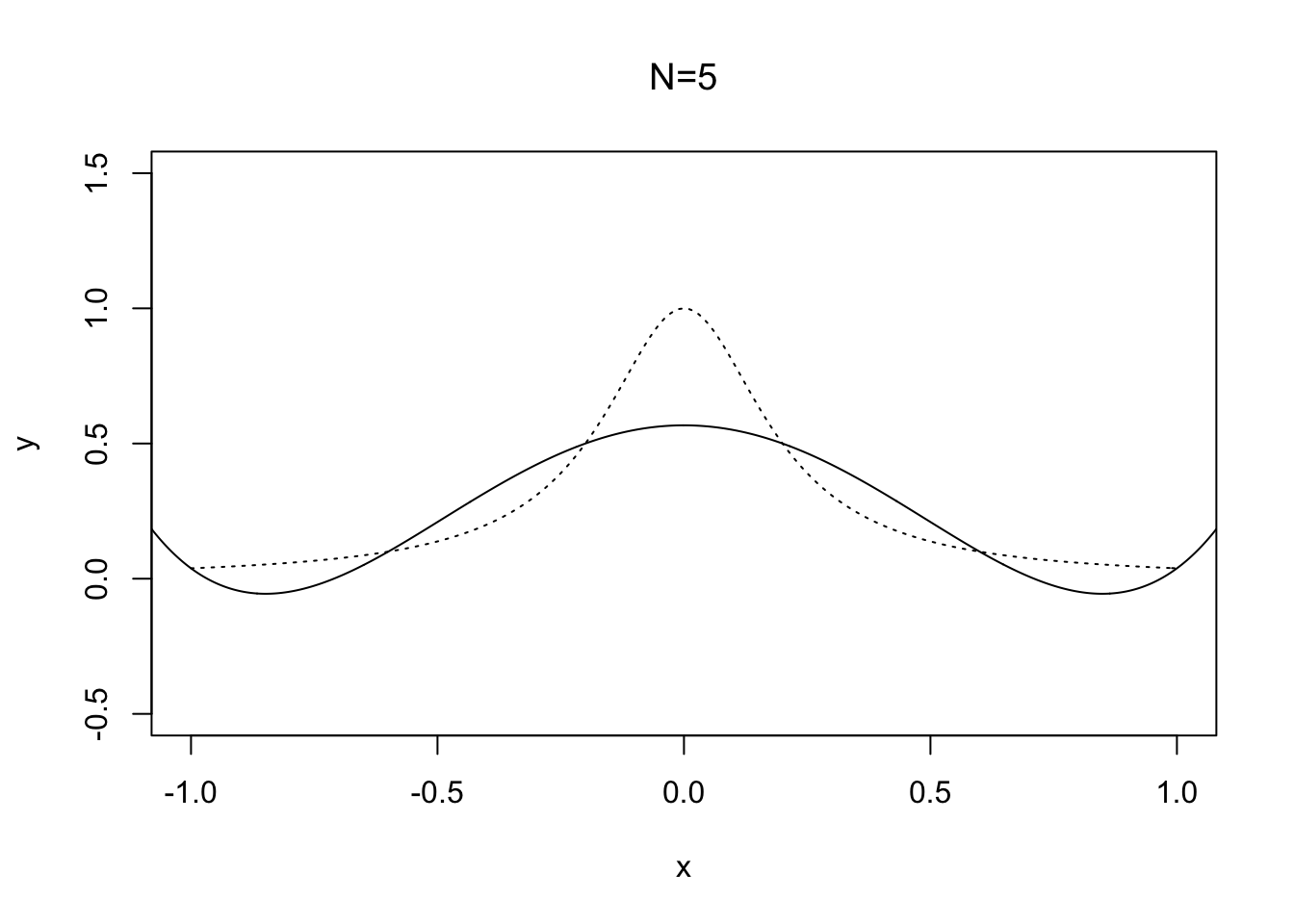
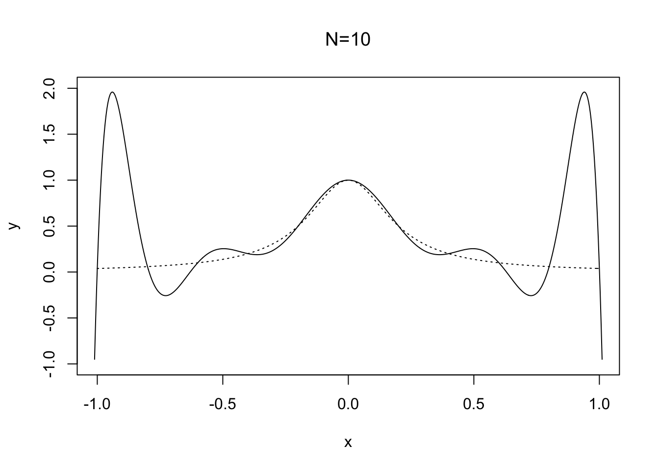
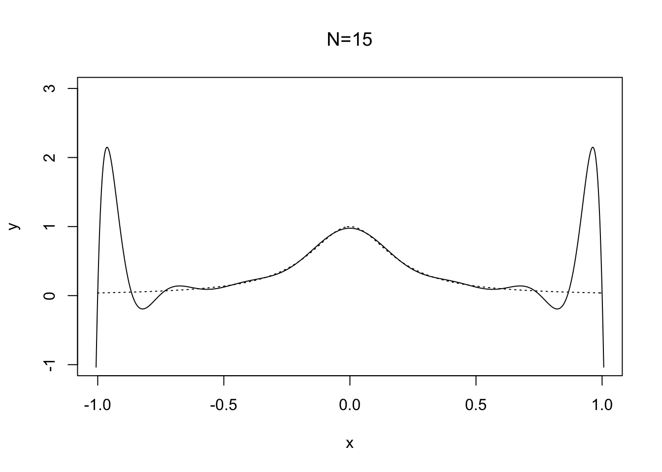
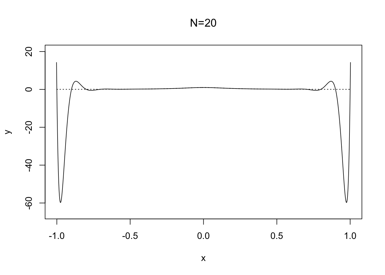
Figure 2.4: Runge’s phenonmenon with the function \(f(x) = 1/(25x^2 +1)\)

Here solid line shows the interpolant \(p_N\in \mathcal{P}_N\) of \(f(x)=1/(25x^2+1)\) based on \(N+1\) uniformly spaced points on the interval \([-1,1]\). Note how the oscillations near the end points become wilder as \(N\) is increased. The difficulty with this choice of \(f(x)\) is its derivatives, which become larger as roughly speaking each derivative increases by a factor of \(25\) and Theorem 2.3 requires the derivatives to be well behaved.

2.3 Newton’s divided-difference formulae

Newton provided an elegant way of writing interpolation formulae, which is especially useful when adding more interpolation points. Let’s derive his divided differences and the associated formulae for polynomial interpolation. We approximate a function \(f\colon \mathbb{R}\to \mathbb{R}\).

One data point We are given \((x_0,f(x_0))\) and the constant interpolation function is \(p_0(x)=f(x_0)\).

Two data points Given a second point \((x_1, f(x_1))\), we wish to update the interpolation function by increasing the polynomial degree. We write \[ p_1(x)=p_0(x)+A_1 (x-x_0), \] where \(A_1\) is a coefficient to be determined. Notice that \(p_1(x_0)=f(x_0)\) for any choice of \(A_1\); we automatically satisfy the first interpolation condition. To determine \(A_1\), apply the second interpolation condition \(p_1(x_1)=f(x_1)\), to find \[ A_1=\frac{f(x_1)-p_0(x)}{x_1-x_0} = \frac{f(x_1)-f(x_0)}{x_1-x_0}. \] This quantity is Newton’s first divided-difference and usually denoted \(f[x_0,x_1]\) (or \(f[x_1,x_0]\) as order does not matter here). The linear interpolant is \(p_1(x)=f(x_0)+f[x_0,x_1](x-x_0)\).

Three data points Add another data point and build the degree-two interpolant \(p_2(x)\) by adding to the already-known degree-one interpolation. Write \[ p_2(x)=p_1(x)+A_2(x-x_0)(x-x_1) \] for some \(A_2\) to be determined. Notice that \(p_2(x)\) satisfies the first two interpolation conditions, and \(A_2\) is determined by \(p_2(x_2)=f(x_2)\). That is, \[ f(x_2)=p_1(x_2)+A_2(x_2-x_0)(x_2-x_1)\] so that \[ A_2 =\frac{f(x_2)-f(x_0)-f[x_0,x_1](x_2-x_0)}{(x_2-x_0)(x_2-x_1)} = \frac{f[x_2,x_0]-f[x_0,x_1]}{(x_2-x_1)}=\colon f[x_0,x_1,x_2], \] which is the second Newton divided-difference. You should verify that permuting \([x_0,x_1,x_2]\) leaves its definition unchanged. The quadratic interpolant \(p_2(x)=f(x_0)+f[x_0,x_1](x-x_0)+f[x_0,x_1,x_2](x-x_0)(x-x_1)\).

Four data points The pattern continues. For example, if we add a fourth point \(x_4,f(x_4)\), the degree-three interpolant is written \[\begin{align*} p_3(x)&=f(x_0)+f[x_0,x_1](x-x_0)+f[x_0,x_1,x_2](x-x_0)(x-x_1)\\ &\qquad+f[x_0,x_1,x_2,x_3](x-x_0)(x-x_1)(x-x_2), \end{align*}\] where the Newton divided-difference is defined by \[ f[x_0,\dots,x_n] \colon= \frac{f[x_1,\dots,x_n]-f[x_0,\dots,x_{n-1}]}{x_n-x_0}, \] which is invariant to permutation of its arguments.