For the purpose of data compression in scientific computing, we use the term “tensor” for any array with many indices. Given a multivariate function \(f(x_1,\ldots,x_d)\), after its independent discretisation in each variable we obtain discrete values which we can collect to a tensor \(F\) and enumerate as \(F(i_1,\ldots,i_d)\). We write the indices in brackets instead of sub- or superscripts to emphasise that they have no additional attributes, on the contrary to e.g. upper and lower indices of tensors in physics. In the previous section we concluded that we should avoid the independent discretisation, so where is the trick? The point is that we will never work with the full tensor \(F\) directly. Instead, we approximate every entry of \(F\) by a mapping of other tensors, which require (much) fewer elements to store.
This story can start already from two dimensions. On the functional level, recall the Fourier method for solution of PDEs with separation of variables. Having, for example, an equation \(\frac{\partial u}{\partial t} = \frac{\partial^2 u}{\partial x^2}\), we seek for a solution of the form \(u(t,x)=\sum_{i}A_i(t)\sin(\lambda_i x)\). Notice that \(t\) and \(x\) appear in different factors, i.e. they are separated.
Those preferring the language of linear algebra may recall that any matrix \(A\in \mathbb{R}^{n\times n}\) with \(\mathrm{rank}A=r<n\) can be written as a product \(A=UV^\top\), where \(U,V \in \mathbb{R}^{n\times r}\). Moreover, we can choose a very particular representation, if the matrix is not of rank \(r\) exactly. Computing the Singular Value Decomposition (SVD) \(A=\hat U \hat S \hat V^\top\) and picking only the dominant components to \(U=\hat U(:,1:r)\hat S(1:r,1:r)\) and \(V=\hat V(:,1:r)\), we end up with an optimal approximation:
$$
\|A–UV^\top\|_2 = \min_{\mathrm{rank}B = r} \|A−B\|_2.
$$
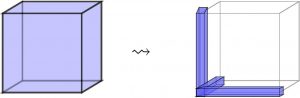
You probably noticed already the way to data compression: instead of storing all \(n^2\) elements of \(A\), we can store only \(2nr\) elements of \(U\) and \(V\). Here is more motivation: if \(A\) is populated by discrete values of a smooth enough function, it can be proven that the error decays rapidly with the rank, e.g.
$$
\|A–UV^\top\|_2 \le C \exp(-\beta r^\gamma).
$$
For tensors with more than two dimensions, it is convenient to write indices explicitly. The matrix low-rank decomposition can be written in the form
$$
A(i,j)=\sum_{\alpha=1}^{r} U_\alpha(i) V_\alpha(j).
$$
Here we put \(\alpha\) to subscript only to show that it is an auxiliary index. A straightforward generalisation to tensors may read
$$
A({\bf{i}})=\sum_{\alpha=1}^{r} U^{(1)}_{\alpha}(i_1)\cdots U^{(d)}_{\alpha}(i_d),
$$
where \({\bf{i}}=(i_1,\ldots,i_d)\). This representation, called CP, CANDECOMP or PARAFAC decomposition is indeed very popular in data science, in particular due to its uniqueness properties (see this review). There are however drawbacks: there is no optimality like with SVD, moreover, the error minimiser may not exist in the set of rank-r CP representations. Computationally more pleasant are the so-called tree tensor formats. The simplest representative of such was rediscovered multiple times, and therefore has multiple names: Matrix Product States, Density Matrix Renormalisation Group, and Tensor Train format. Its general formula reads
$$
A({\bf{i}})=\sum_{\alpha_0,\ldots,\alpha_d=1}^{r_0,\ldots,r_d} U^{(1)}_{\alpha_0,\alpha_1}(i_1)\cdots U^{(d)}_{\alpha_{d-1},\alpha_d}(i_d).
$$
The total storage reduces from \(\mathcal{O}(n^d)\) degrees of freedom to \(\mathcal{O}(dnr^2)\) which is much smaller and most importantly linear in \(d\). The TT-format comes with a full set of cheap algebraic operations and a re-factorisation (truncation) procedure to avoid excessive growth of the ranks \(r_k\).
However, a direct application of this procedure is still impossible in high dimensions, unless the tensor is already available in some factored form. We simply cannot access all \(n^d\) entries to perform an SVD. An alternative is the Cross approximation algorithms, based on incomplete Gaussian elimination. If a matrix admits a low-rank approximation in principle, few steps of \(LU\) decomposition with pivoting often define a very accurate low-rank approximation. Using recurrent extensions of this idea to higher dimensions leads to cross approximation algorithms in tensor formats.
The idea of recurrent application of matrix methods to higher dimensions is used a lot in tensor computations. For example, replacing the pivoting of the cross method by a Galerkin projection onto TT blocks from the previous iteration allows to solve linear equations and eigenvalue problems. These techniques are called alternating iterative methods (not to be confused with Alternating Direction Implicit, although is does have similar concepts). In each step they recompute one block of a tensor format, keeping the others fixed, then do the same on the next block, and so on until convergence.
More information on tensor decompositions and algorithms can be found in a recent book by W. Hackbusch and reviews.