Vibration laboratory

Introduction

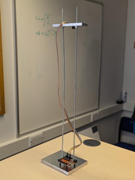
In this laboratory you will be conducting experiments to gather data from the simple vibrating structure shown in , and then mathematically analysing the data in order to generate a representative one-degree-of-freedom model for the system.

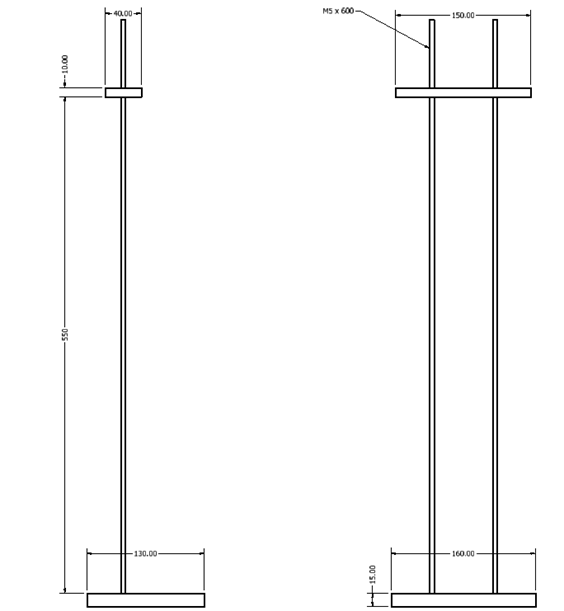
The vibrating system is made up of four components, a base and top piece made of Aluminium 1050 and two steel M5 threaded rods each approximately 600 mm long. The top piece is held in place by nuts and washers at an approximate position of 550 mm above the base plate.

A three-axis accelerometer (Analog Devices MMA8451) is attached to the top piece in order to measure the motion of the structure, this connects to an Arduino for data logging as shown in .

The aim of this lab is to give you hands on experience with the theoretical concepts covered at the beginning of the course and help you understand the use of 1DOF vibrations as taught so far but also its limits when applied to real world problems. There are three objectives:

1. Examine the difference between the calculated and measured parameters of a simple vibrating structure.
2. Confirm the relationship between natural frequency and mass.
3. Investigate how a pendulum can act as a vibration absorber for the vibrating structure (The theory for this should be covered in the vibration of two degree of freedom systems).

Theory

The standard equation of a 1DOF mass-spring-damper system is given as:

where $\omega_n$ the undamped natural frequency is:

and the damped natural $\omega_d$ is:

From the free vibration response of the system, the damping ratio $\zeta$ may be estimated from the logarithmic decrement:

where $x_1$ and $x_2$ are the amplitudes of the two consecutive peaks.

For low damping $\zeta \ll 1$, $\ln \left(\frac{x_1 }{x_2 }\right)\approx 2\pi \zeta$ and the damping may be estimated as:

For a simple pendulum of length $L$, the frequency of oscillation is given as:

It can be shown (see Vibrations of multi-degree of freedom systems) that a pendulum mounted on the structure in can be tuned to act as a vibration absorber where excitations applied to the structure are fully transmitted to the pendulum.

The task

Working in groups of two or three, you will have your own vibrating structure and data logging setup to complete this lab, you can collect and process as much data as you would like during the 90 min session. Therefore the procedure laid out below can be seen as a scaffold for your experimentation rather than a tick list:

1. Confirm you are able to log data in line with the instructions provided for setting up the experiment. Confirm the measured values are sensible!
2. Record free vibration responses and measure the natural frequency of the vibrating structure.
3. Take any physical measurements of the structure that may be relevant for the theoretical calculations of some system parameters.
4. Add 200g to the structure and repeat the above step 2 (this will allow you to decompose the stiffness and mass later).
5. Add the pendulum and use the natural frequency and pendulum equation to sets its length to maximise vibration absorption.
6. Empirically tune the pendulum length and analyse the effect on the vibration of the structure.
7. Run any other tests you would like within the 90 minutes.

Set-up instructions

Start by downloading the MATLAB and SIMULINK files required for this lab.

1. Connect the Vibrating Frame Arduino to a desktop USB port.
2. In the desktop “Device Manager”, identify the port of connection ‘COM#’ of the Arduino.
3. Open the file Vibration_Lab_MMA_setup.m and change the COM port in the first line “a = arduino(‘COM#’, ‘Uno’, ‘Libraries’, ‘I2C’)” replacing COM# by the number identified in step 2.
4. Run the file “Vibration_Lab_MMA_setup.m” in MATLAB to initialise the accelerometer MMA8451.
5. Open the file “Vibration_Lab_Datalog.slx” in Simulink.
6. On the Simulink menu, select the Hardware Tab and then click on Monitor & Tune to run the data acquisition code.
7. Double click on the “Scope” to observe the data acquisition and apply an initial disturbance on the vibrating frame.
8. At the end of the 20 seconds data logging, enter relevant comments in the “Experimental notes:” in the MATLAB command window.
9. Repeat steps 6 to 8 for all the experiments that are required in lab sheet experimental procedure.
10. At the end of the session, in the Home Tab of the MATLAB menu, click on Save Workspace to save all your experimental data with the relevant_name.mat.
11. Later, you should be able to retrieve all your experimental data by opening MATLAB and running the following command load ‘relevant_name.mat’. Or alternatively clicking on Import Data and selecting your file relevant_name.mat

Once this is done you should be able to plot all the graphs recorded during experimentation and process your data to determine various parameters as required in the lab sheet.

Taking data

The data gathered can be viewed by double clicking on the scope, which gives a display of the type shown in Figure 3.

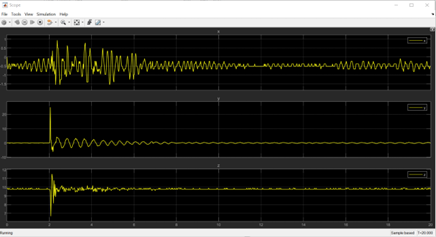
At the end of each test you will be prompted to add any notes to the data and then it will be stored in the MATLAB workspace in a variable named Testn where n is an incrementing counter. For example to plot the data from this first test of the apparatus.

plot(Test1.time,Test1.data)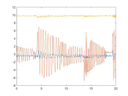

plot(Test1.time,Test1.data(:,2))

xlim([2 8])
ylim([-15 15])
formatplot('Time (s)','Y Acceleration (m /s^2)')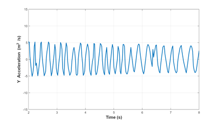

After the lab session

Key points to consider:

• Calculate the expected theoretical natural frequency and its derivation (using measured dimensions and material properties).
• Use the change in natural frequency with an increase in mass to find the representative stiffness and mass, how do these compare to you calculations? If they are different why?
• Report the change in damping ratio observer when the pendulum was added.
• Investigate how the length of pendulum affect the response of the vibrating frame. Is there an optimal damping depending on the pendulum length?
• Identify any experimental errors or unexpected trends and their possible sources.

Functions for plotting graphs

function formatplot(xtitle,ytitle,varargin)

grid on

xlabel(xtitle,'fontsize',14,'fontweight','bold');
ylabel(ytitle,'fontsize',14,'fontweight','bold');

set(gcf,'Position', \[0 0 960 540\]);

h = findall(gcf,'Type','Line'); set(h,'LineWidth',2);

if nargin ==3 legend(cellstr(varargin1)) legend boxoff elseif nargin \>=
4 legend(cellstr(varargin1),'Location',varargin2) legend boxoff end

end