Modelling Wireless Power Transfer in Ansys

In this lab we will simulate wireless charging coils using Ansys Electronics Desktop. We will begin with some basic wireless charging theory where we define a model and some parameters of interest.

In Section 1, we will go step-by-step through the simulation of a simple coreless wireless power system, including geometry setup, boundary conditions, meshing, excitations and analysis setup. We will also look at how to analyse the simulation results including graphing and visualising fields. The modelling activity in Section 1 can be used to claim the associated skill at Knowledge level.

In Section 2, we will look at a ferromagnetically cored wireless charging system to compare it to the coreless system. The work in Section 2 can be used to claim the associated skill at Application level.

The Lab is associated with the Design Skill: Finite Element Analysis, which you should complete in your Mahara Portfolio.

Wireless Power Transfer Theory

Wireless power transfer can be achieved in several different ways, including with acoustic fields (ultrasonic), optical fields (lasers) and electric fields (capacitive transfer). The most common, used for charging smartphones and other consumer devices, is with magnetic fields (inductive power transfer). An inductive power transfer system works by driving an AC current into a transmitter coil, which produces an AC magnetic field in the space around it, which in turn induces a voltage nearby receiver coil, facilitating power transfer.

We can model an inductive power transfer system as a simple coupled inductor network seen in or a 2-port network model in :

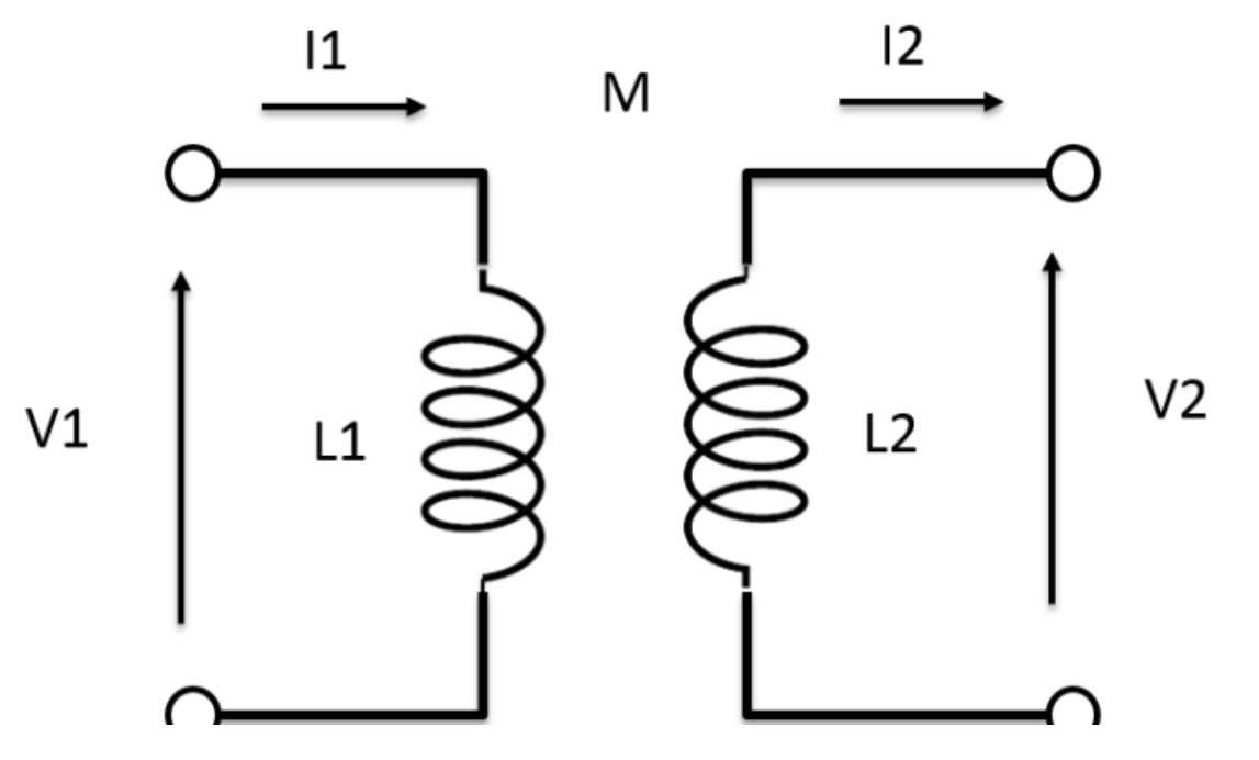
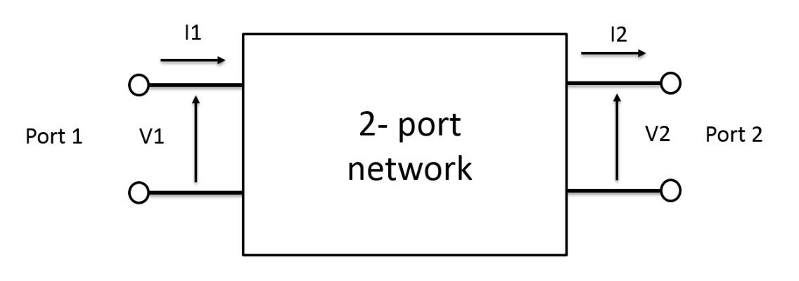
Where V1, I1 are the current and voltage in the transmitter coil and V2, I2 are the current and voltage in the receiver coil.

We can also express this in terms of an Impedance Matrix:

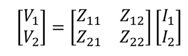
Where $Z_{11}$ is the complex impedance of the transmitter coil, $Z_{22}$ is the complex impedance of the receiver coil and $Z_{12} = Z_{21}$ is the complex mutual impedance between the two coils. $M$ is the mutual inductance between the coils.

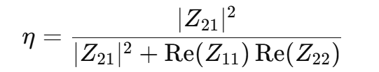
With a set of physical constraints, we want to maximise the power transfer efficiency, which can be approximated by:

When we design our transmitter and receiver coils, we can choose from a near-infinite combination of geometries (coil and wire radius, cross-section, shape, number of turns, turn-spacing) and materials (100s of types of ferrites, substrates).

We can use a tool like Ansys to explore our design space using Finite Element Analysis.
 

Section 1: Coreless Wireless Power Transfer System (K)

In this section we will go step-by-step through analysing a coreless (non-ferromagnetically cored) wireless power transfer system.

Solution Type

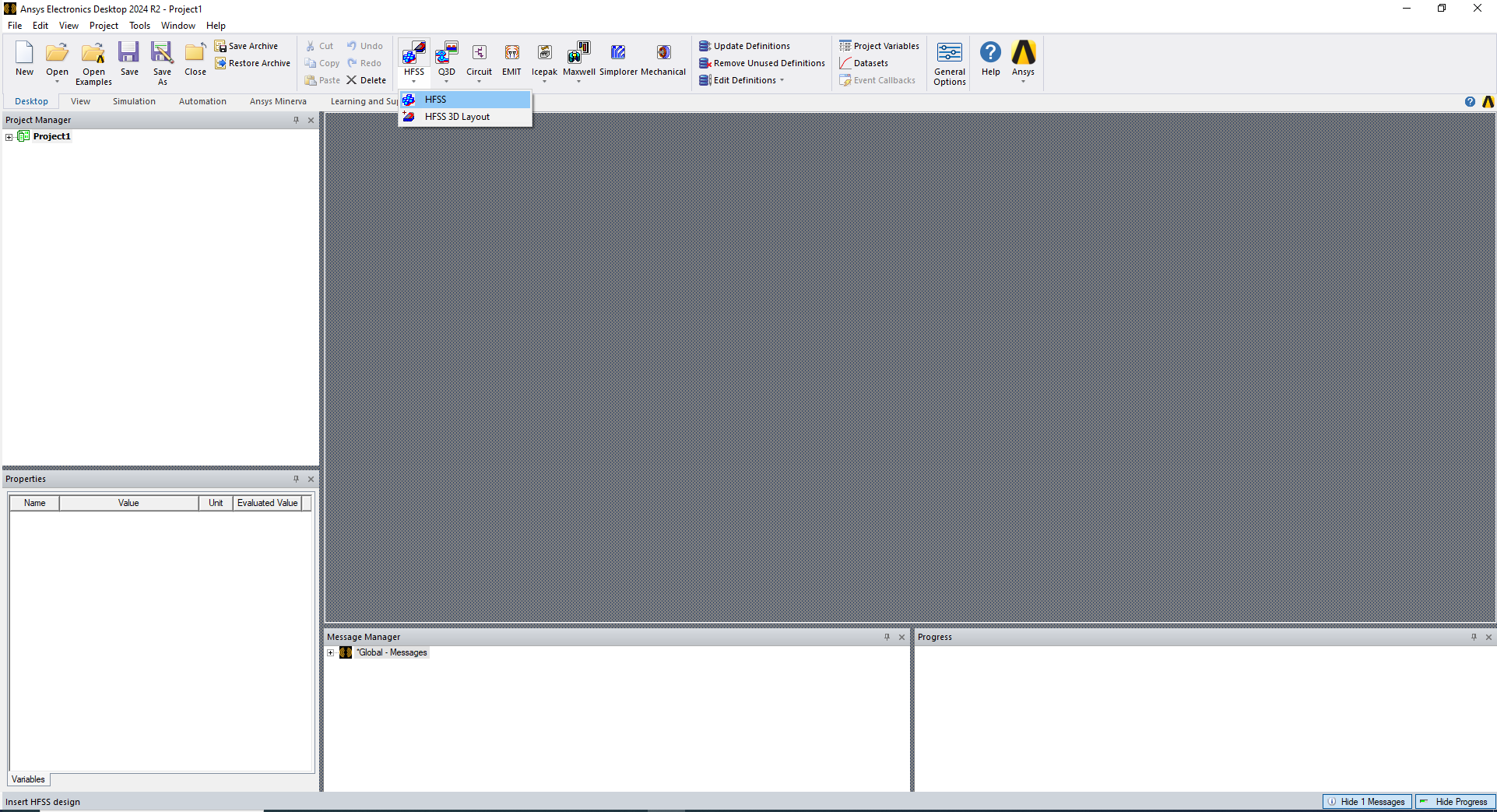
First, open Ansys Electronics Desktop R2 and add a new HFSS Design:

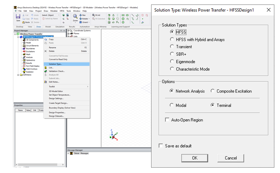
Specify the Solution Type as HFSS, Network Analysis and Terminal:

Creating Coil Geometry

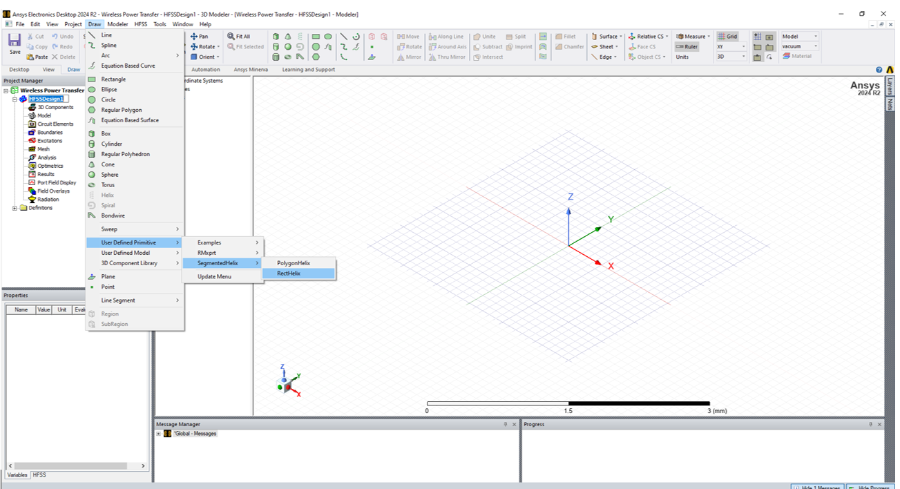
Next, we want to create our coil geometry. To create a coil from scratch most easily, we can add a Rectangular Helix by navigating to Draw » User Defined Primitives » Segmented Helix » RectHelix

We want to add a circular coil of 4 turns and approximate radius of 25 mm with thickness of 100 µm. We also want to approximate the circular coil with 36 segments per turn.

The values in the dialog box below should work:

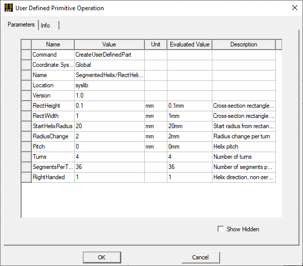
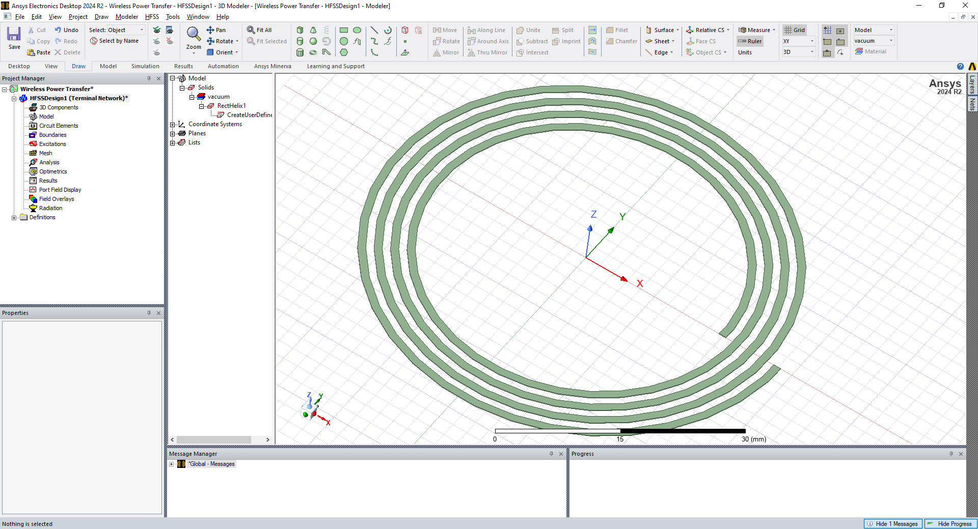
Clicking OK should give a coil that looks like this:

Forming a Closed Loop

We want to simulate driving current through the coil we have made, to see the magnetic field it produces and see how this field will couple to a secondary coil. Current flows in loops, so we need to define how to close the loop.

This is a particularly taxing part of electromagnetic FEA modelling and different solvers/environments take different approaches. In Ansys, we must draw an extension on the coil that we have just made and close the loop using a vector on a 2D plane.

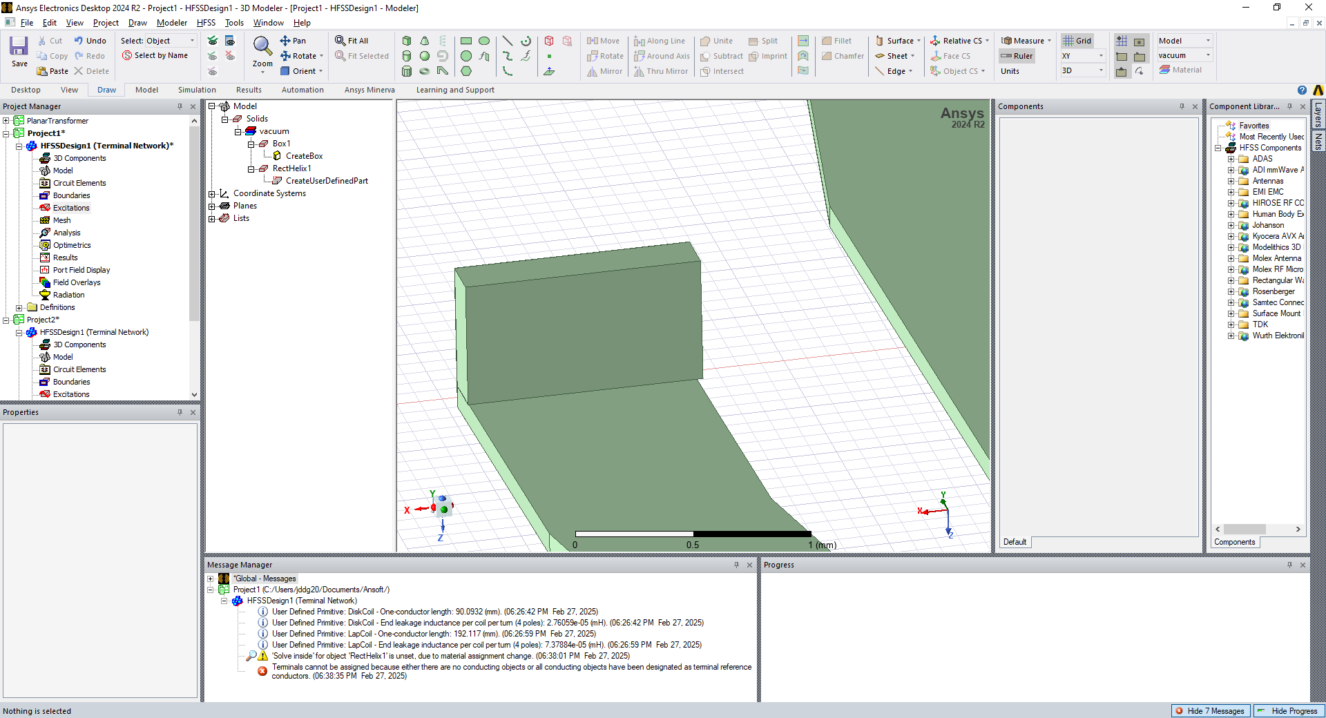
• Zoom into the outermost corner of the coil and select draw box:

• Draw a small box directly on top of the outer part of the coil, which should end up looking like this:

• Select both the coil and the box and select unite:

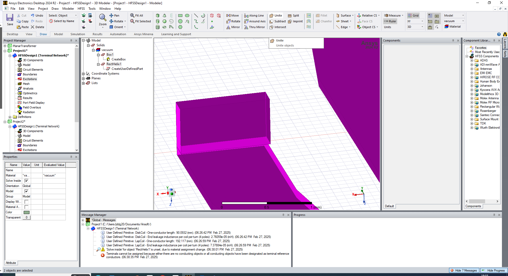
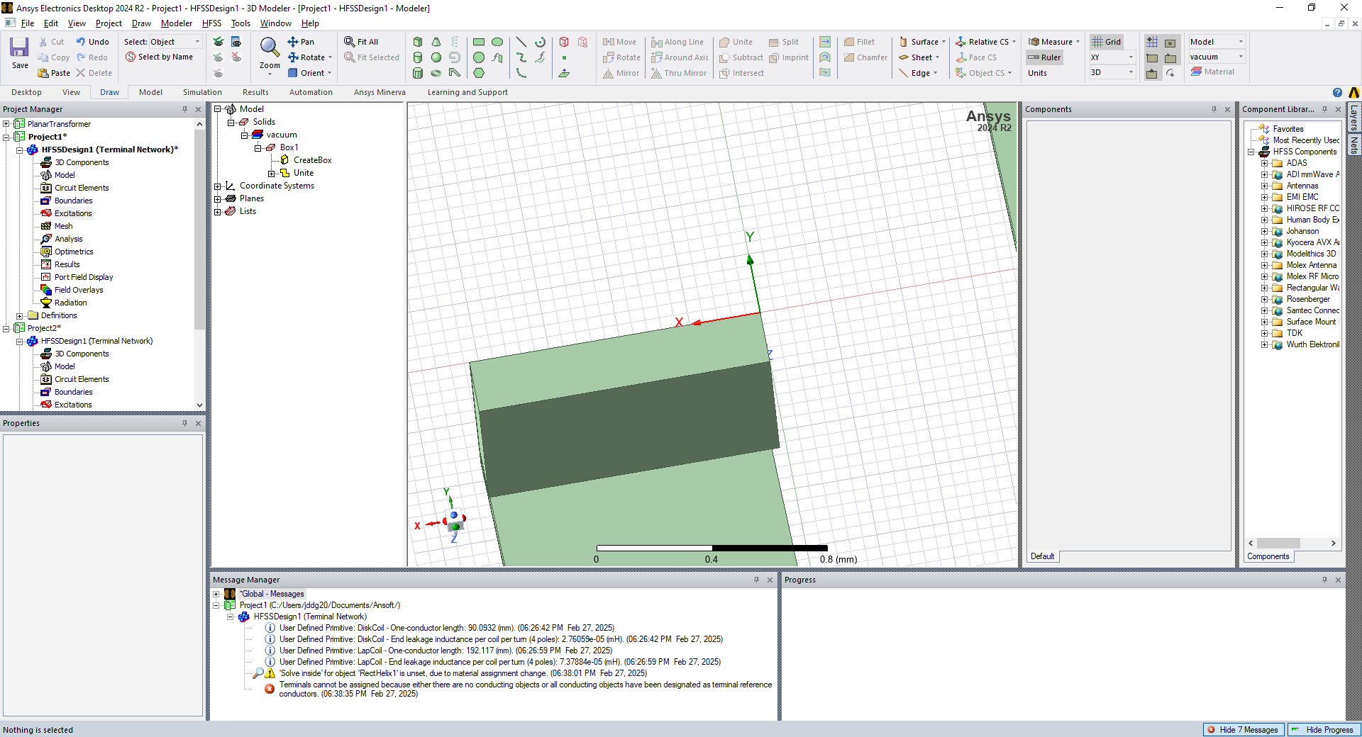
• Use the relative CS button to create a relative coordinate system at the top of the box

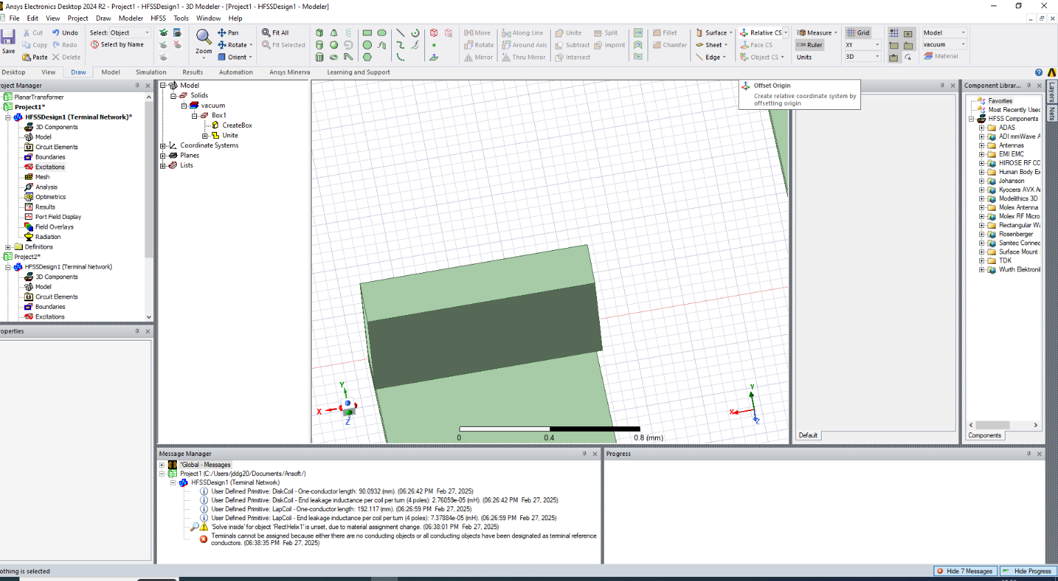
Resulting in a new relative coordinate system on the edge of the rectangle you have just made (which can be edited in the Model tab):

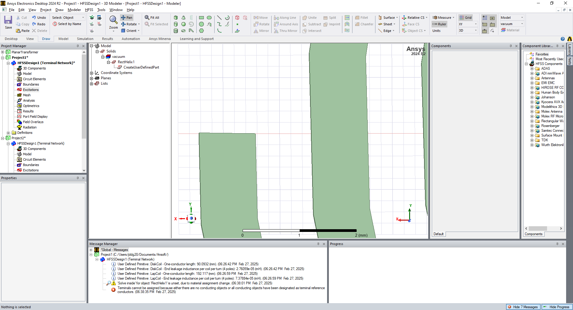
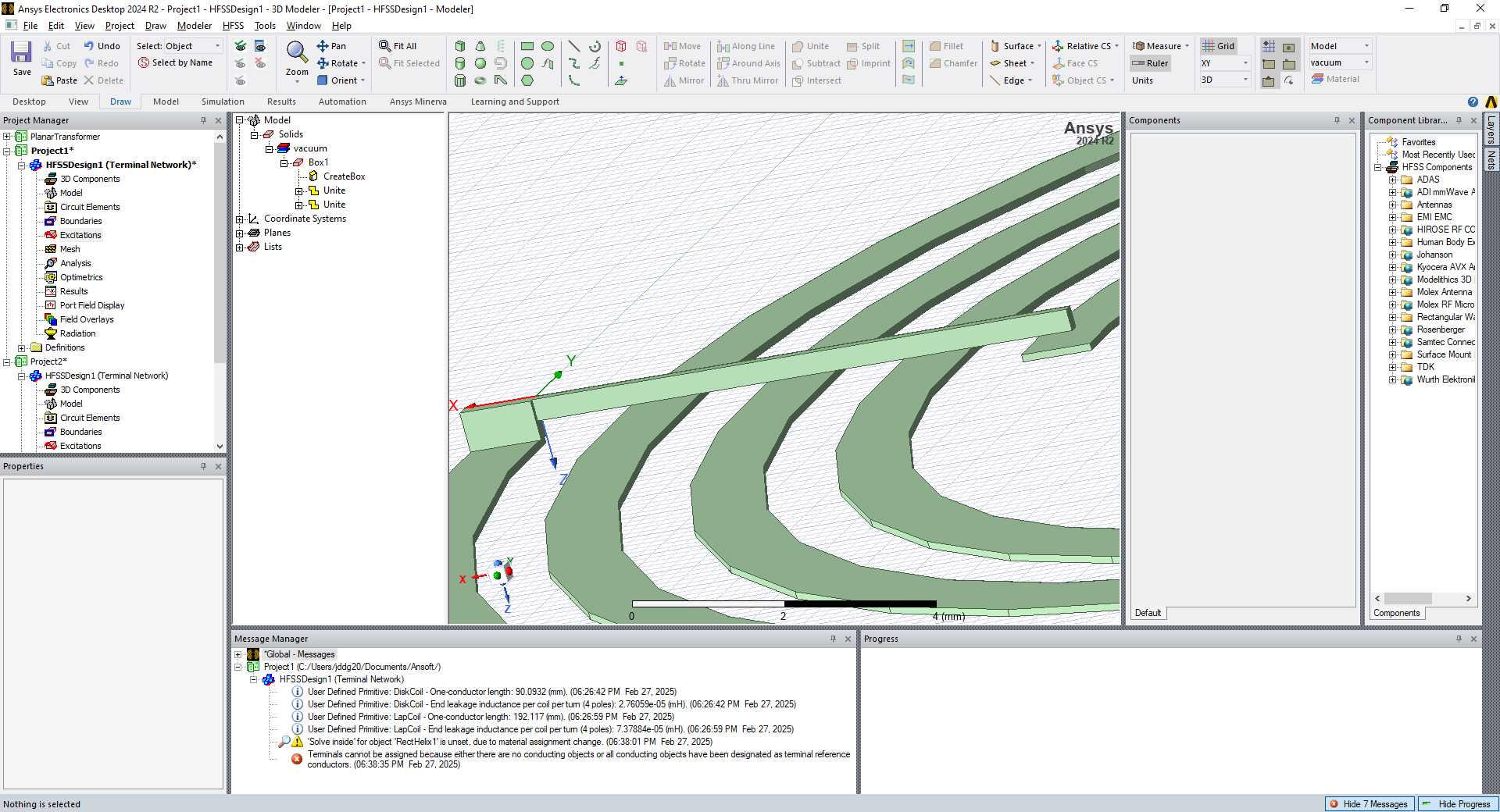
• We now must connect to the other end of the coil. Zoom out slightly and create a long thin rectangle (using draw box again) that reaches over to the interior coil termination. Go ahead and unite this new block with the rest of your coil.

This should now form a single component looking something like:

Assigning Coil Material

Now that we have the basics of the coil that is almost (but not quite) a closed loop, we want to assign a material to the coil.

Select our coil in the modeler (it will show up highlighted in purple), right click and Assign Material:

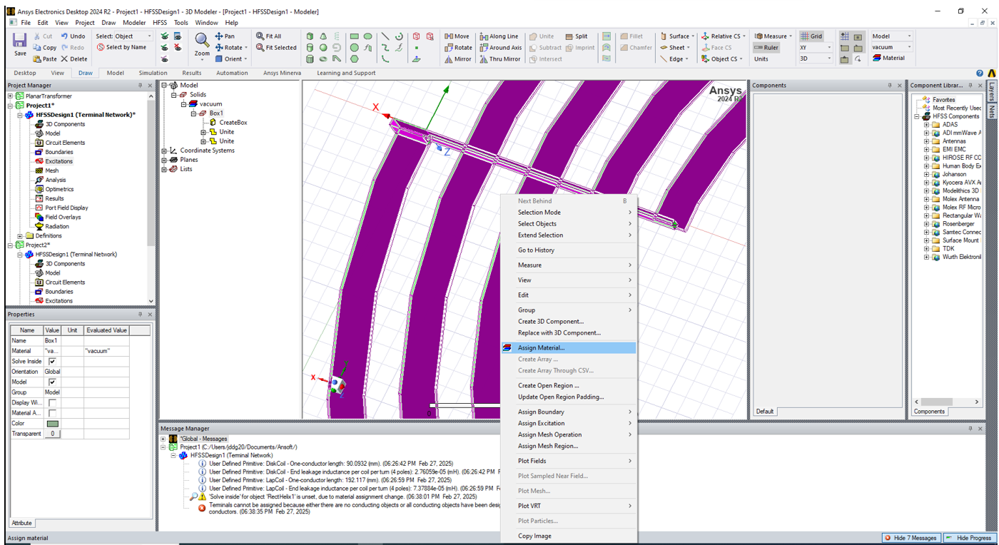
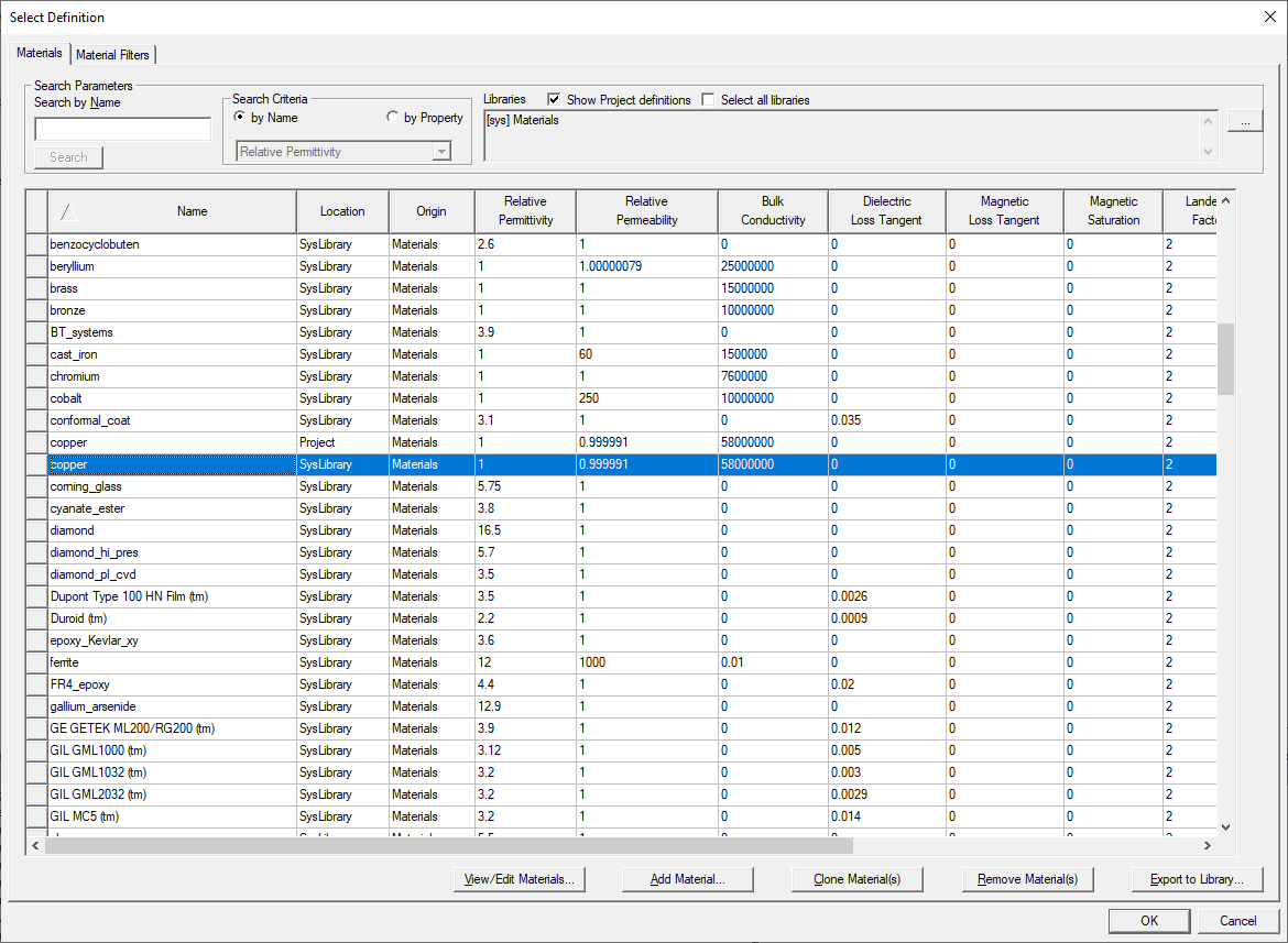
Assign the material as Copper from either the SysLibrary or your project:

Assign Coil Excitation

We now assign the excitation (forcing term) to our coil.

First, we must create a sheet between the two ends of the coil, which acts as an excitation port. Zoom in to the area around the terminations and set another relative CS on the face of one of the coil ends:

Now create a rectangular sheet that completes the circuit between the two coil ends. Use the Draw Rectangle on the main toolbar.

This should end up looking like this:

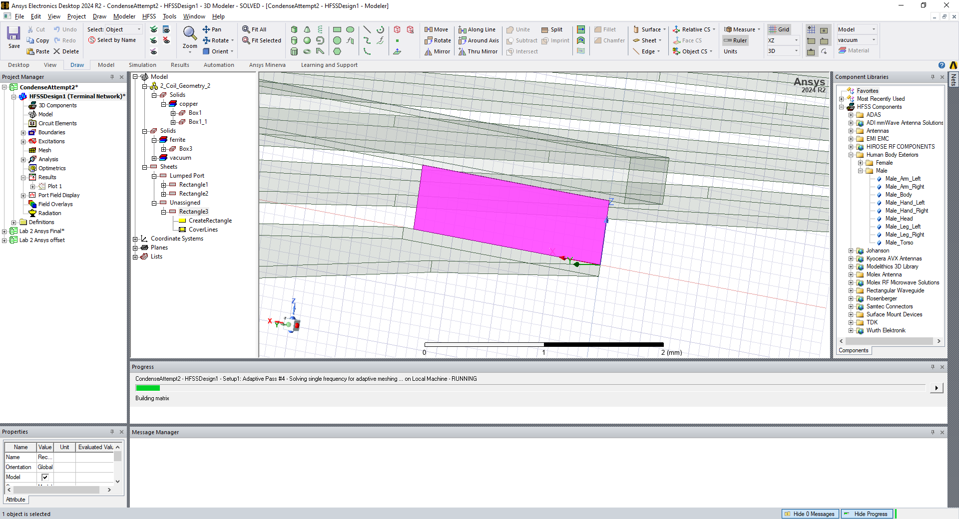
We can now assign an Excitation.

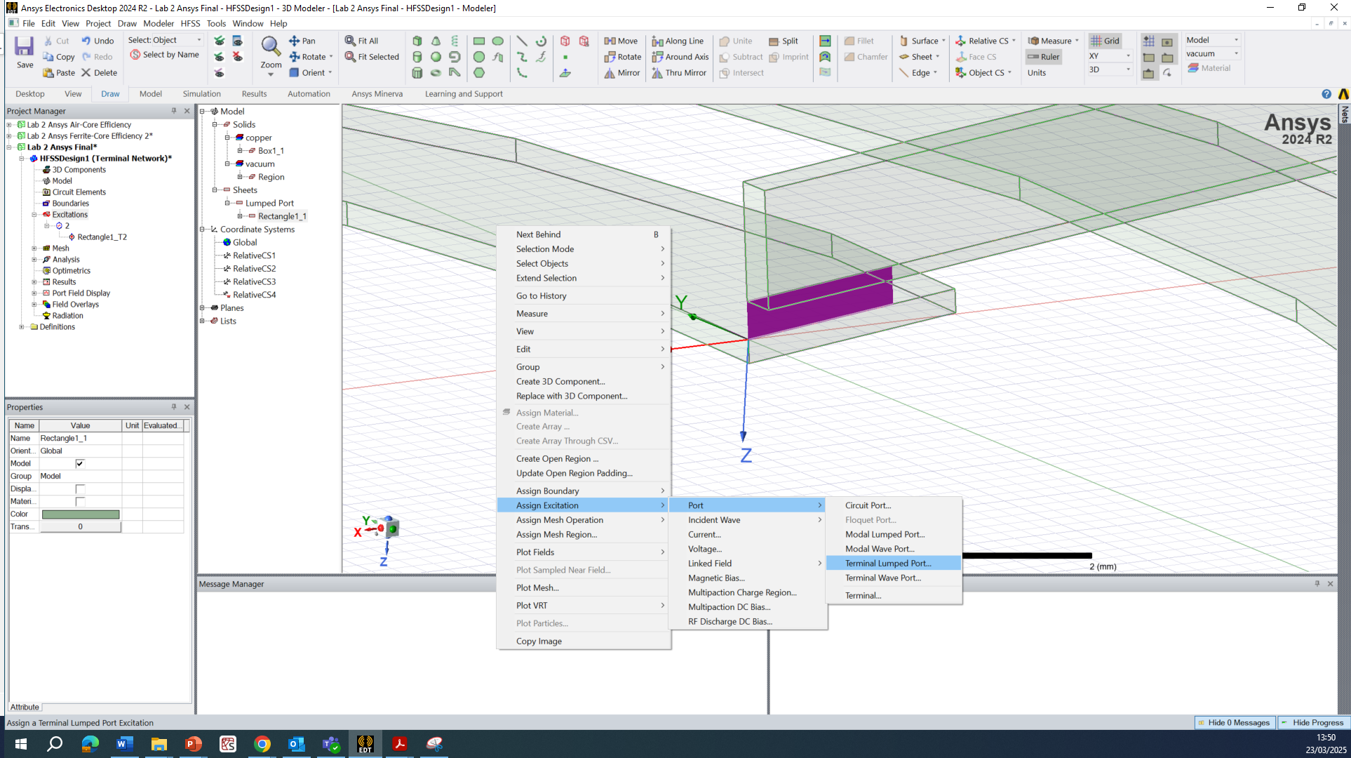
Select the rectangle plane you have just drawn, right click and select Assign Excitation » Port » Terminal Lumped Port…:

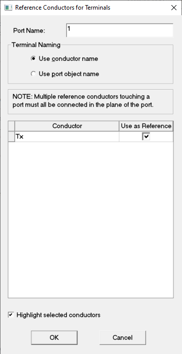
A dialog box should pop up and you should check the ‘Use as Reference’ box for a single conductor. Also, rename the conductor as ‘Tx’ to represent the transmitter coil port. You can rename the port later manually if you like.

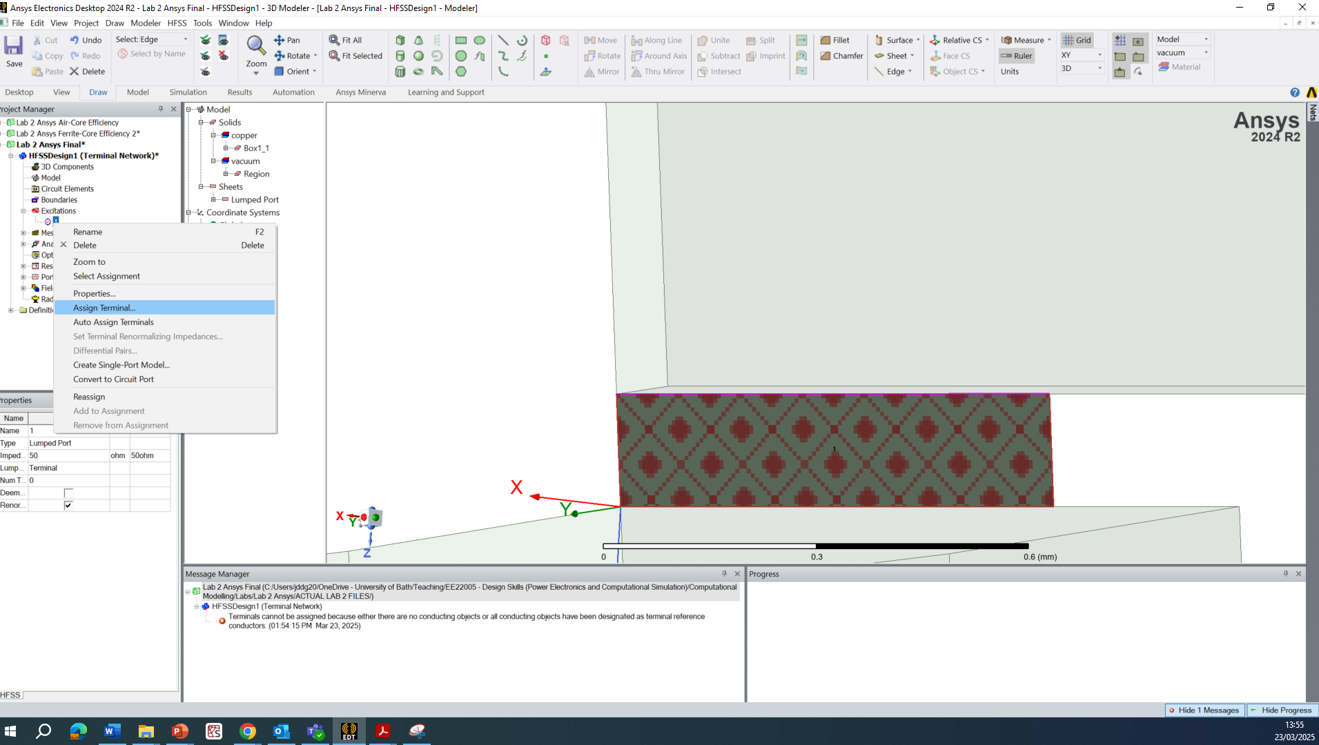
Sometimes this doesn’t work as Ansys is trying to automatically detect the conductor to attach the port to, but the process can fail. If this is the case, you may have to manually assign the port terminal. You can do this by selecting an Edge (press ‘E’ on your keyboard) of the rectangular port and right click on the Port and Assign Terminal:

Building a Receiver Coil

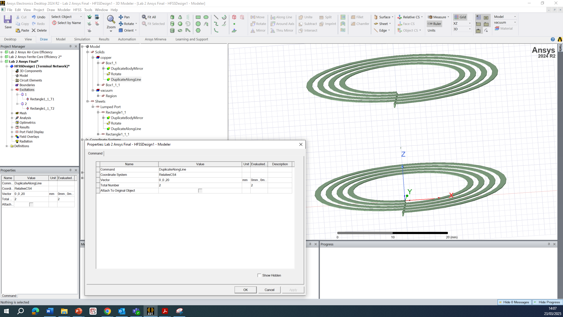
To make a receiver coil, simply duplicate the transmitter coil you have just made.

Do this by selecting all objects (press ‘O’ on your keyboard), remember to select the coil as well as the port and terminal. Then click Duplicate Along Line:

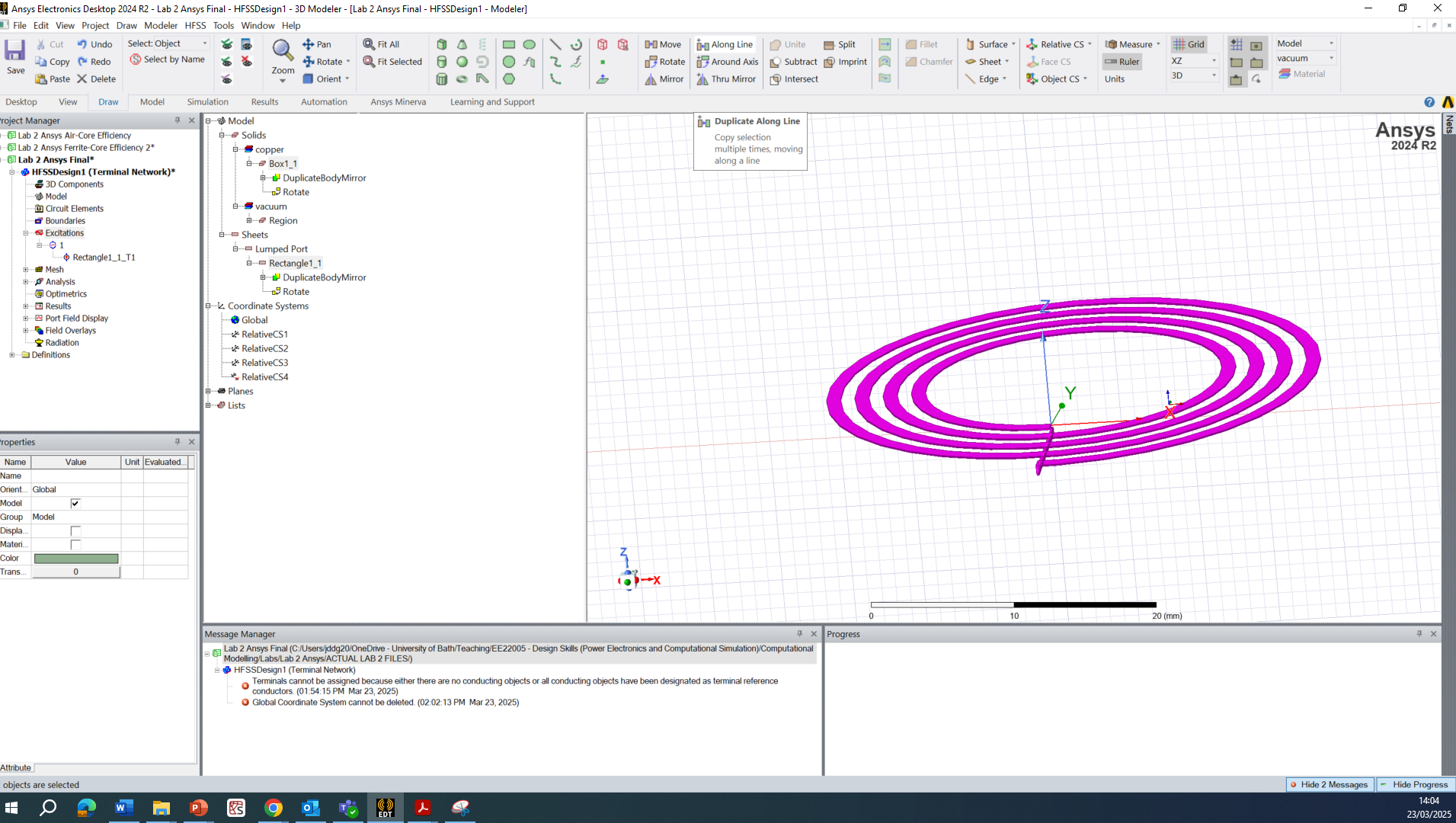
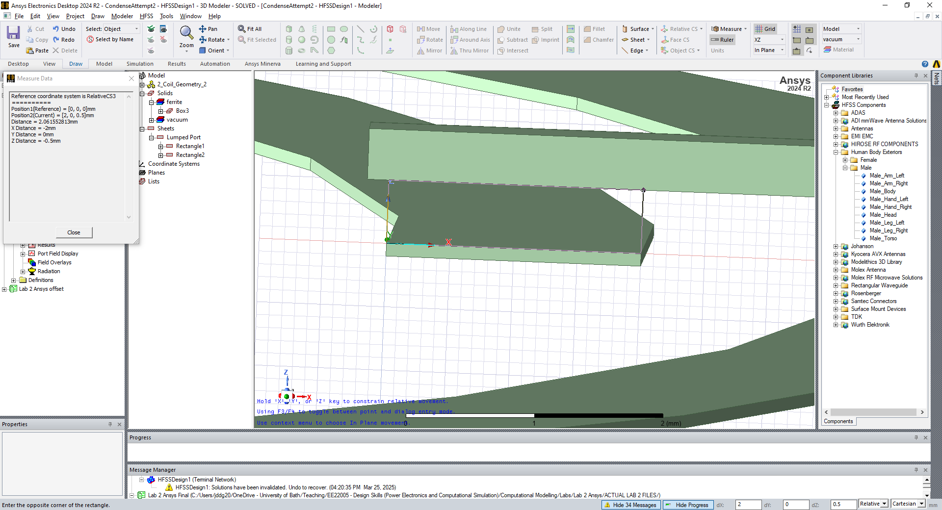
We want the receiver coil to be separated by about 20 mm in the Z direction. The easiest way to do this is just drag the coil in the interactive modeler. This separation doesn’t have to be perfect. You can always edit the duplication in the model editor and the line ‘Vector’ should be 0,0,20.

All going well, you should have something like this:

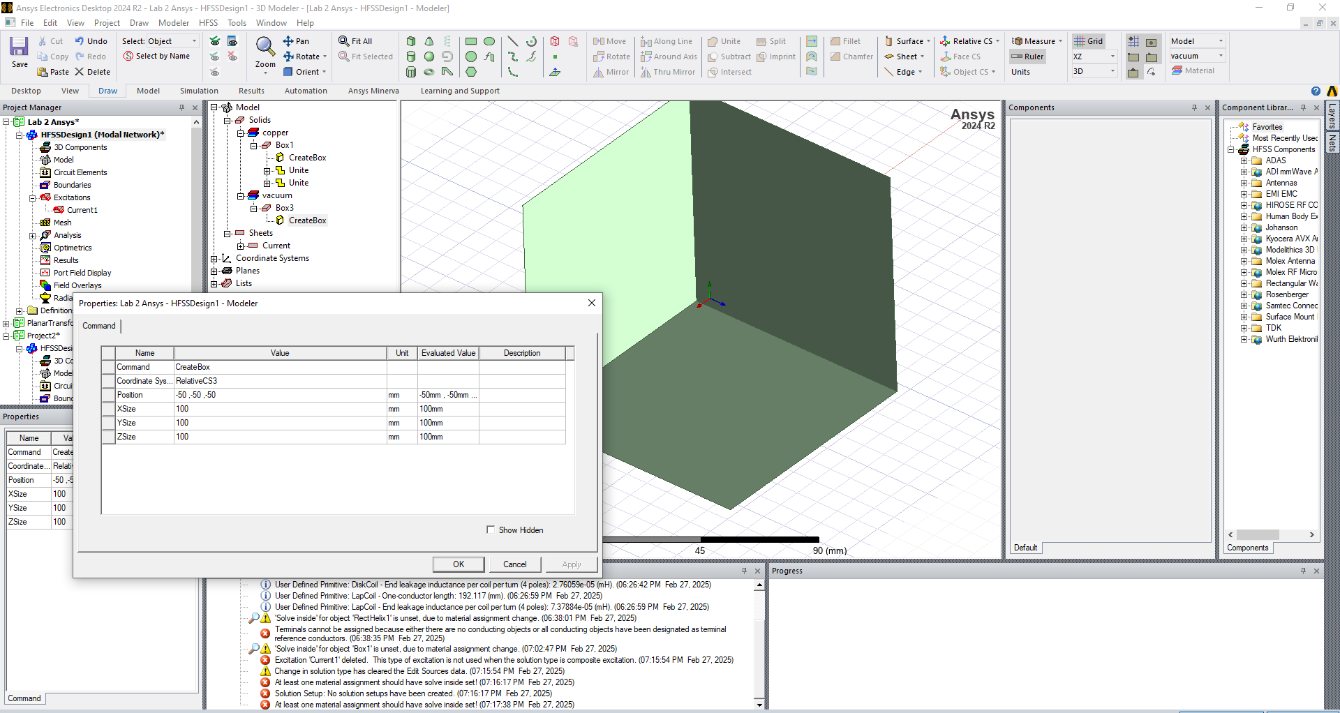
Adding the Vacuum Region and Boundary Conditions

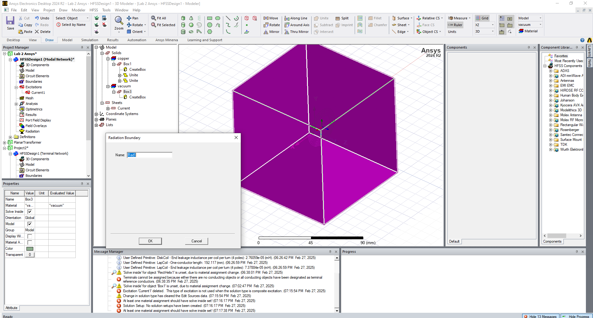
There are several options about how to add boundary conditions. One option is explicitly defining the 3D space we want to solve in. We can do this by creating a box 100x100x100 mm that encompasses the coils and has some space beyond them. You must offset the box so that it surrounds the coils in all directions:

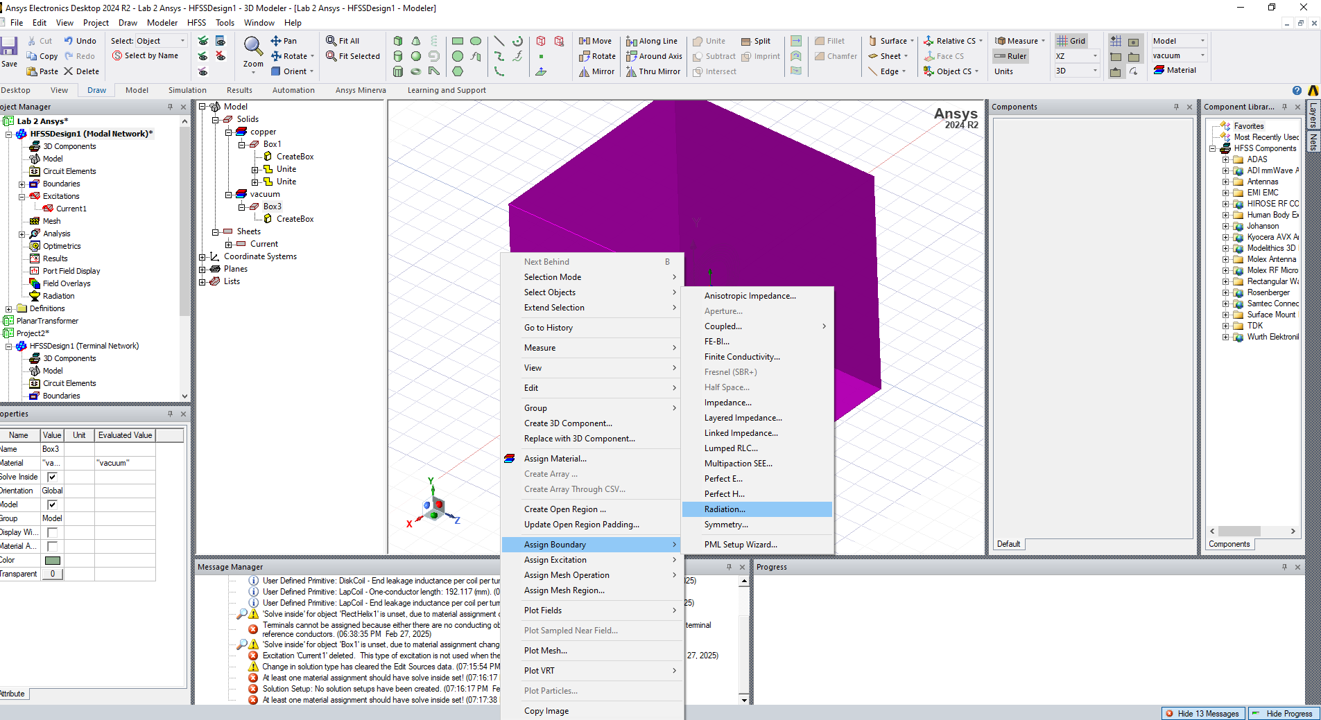
Then select the entire object, right click and select Assign Boundaries » Radiation:

Solver

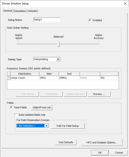
We can now define the analysis. Right click Analysis » Add Solution Setup » Auto…

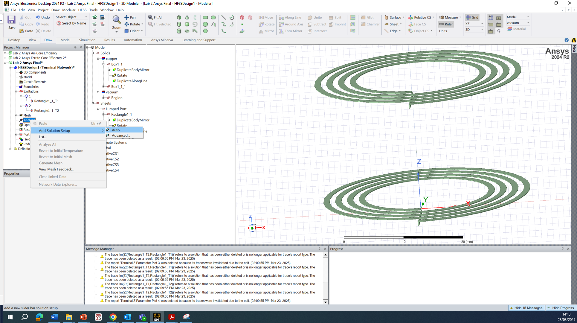
Change the analysis to start at 1 MHz, end at 20 MHz and make sure to check the Save Fields tick box:

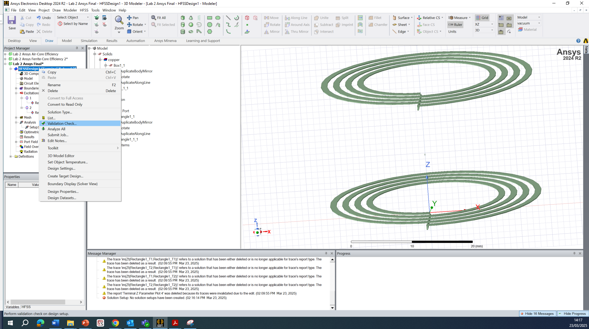
Now right click on you design and select Validate which will hopefully come up with green ticks for each of the preceding steps.

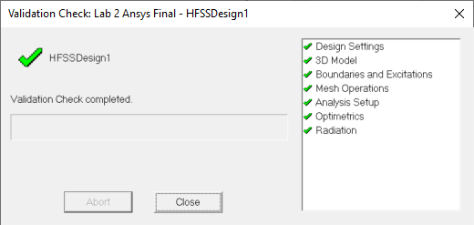
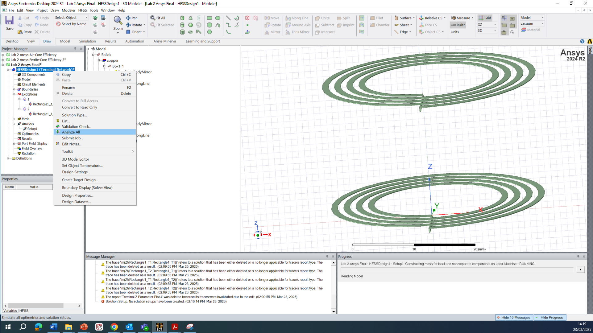
If all is green, congratulations! You can now run the analysis by selecting Analyze All – this should take a few minutes. If it is taking >15 minutes, something has gone wrong, and you may want to review how you have defined your geometry and port definition.

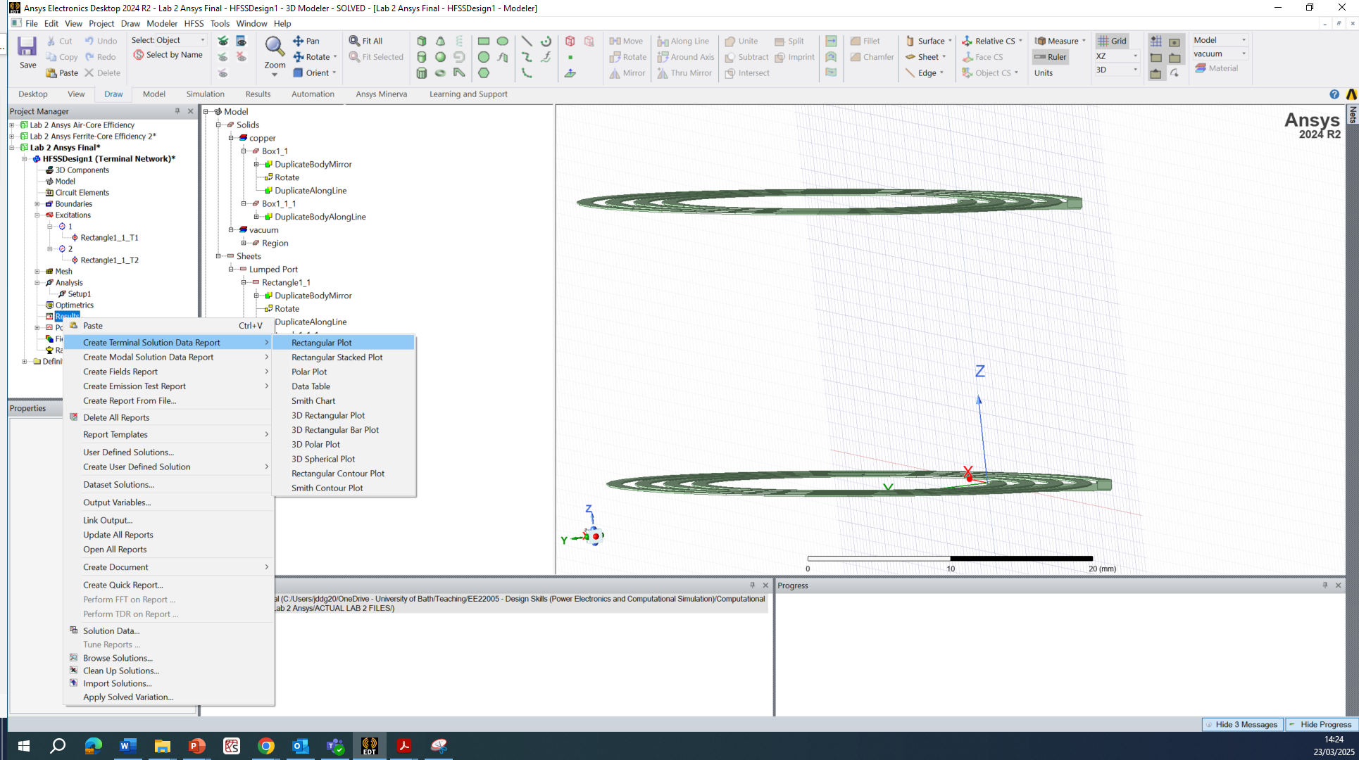
Results

After the analysis has completed, we want to see our results. The most important result is efficiency. To see this, right click Results » Create Terminal Solution Data Report » Rectangular Plot

Recall our expression for efficiency in

We can calculate this by putting the following expression into the ‘Y’ dialog box:

Mag(Zt(Tx,Rx))^2/(Mag(Zt(Tx,Rx))^2+re(Zt(Tx,Tx))*re(Zt(Rx,Rx))) 

Now click New Report and you should see something like the plot in the background:

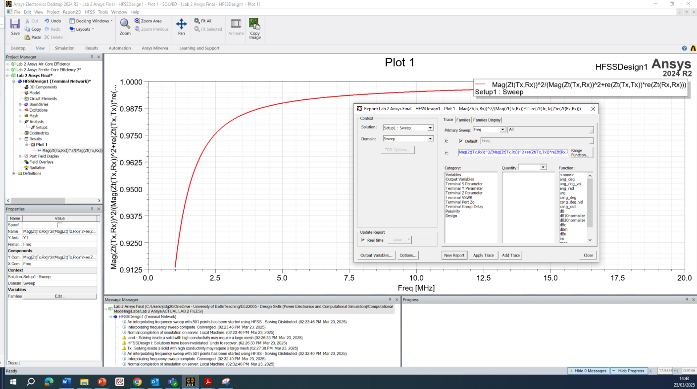
This plots the efficiency vs frequency for this set of coils. As expected from theory, the efficiency increases with increasing frequency.

Getting a result like this is sufficient to claim the skill at Knowledge level – remember to include a screenshot of the setup, comment on the physics being solved as well as the excitations and boundary conditions.

Visualisation (optional)

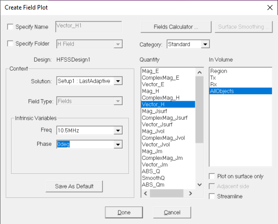
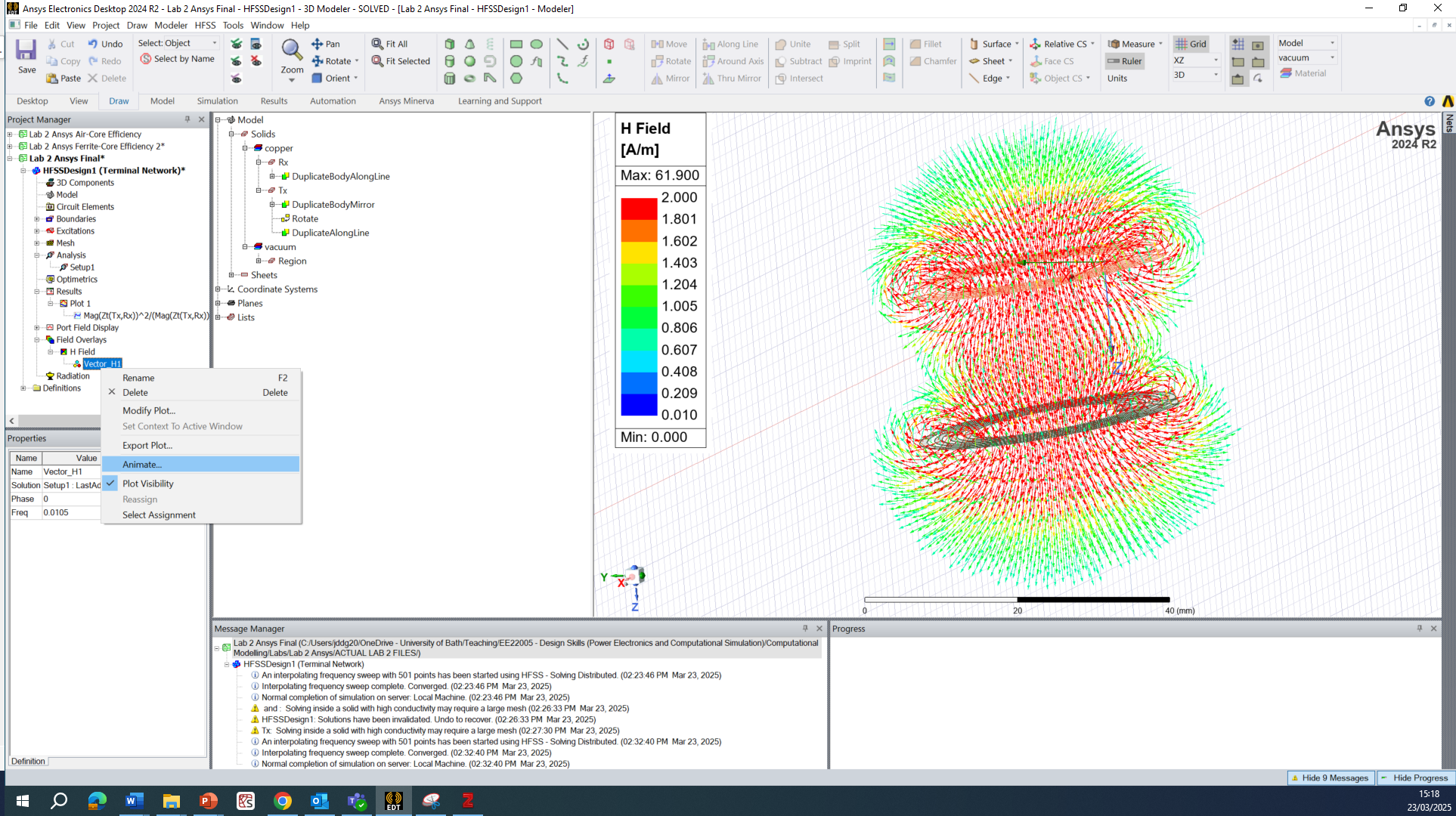
We may also want to view the magnetic fields produced by the coils. To do this, we select the Region that we want to see them, right click and select Plot Fields » H » Vector_H

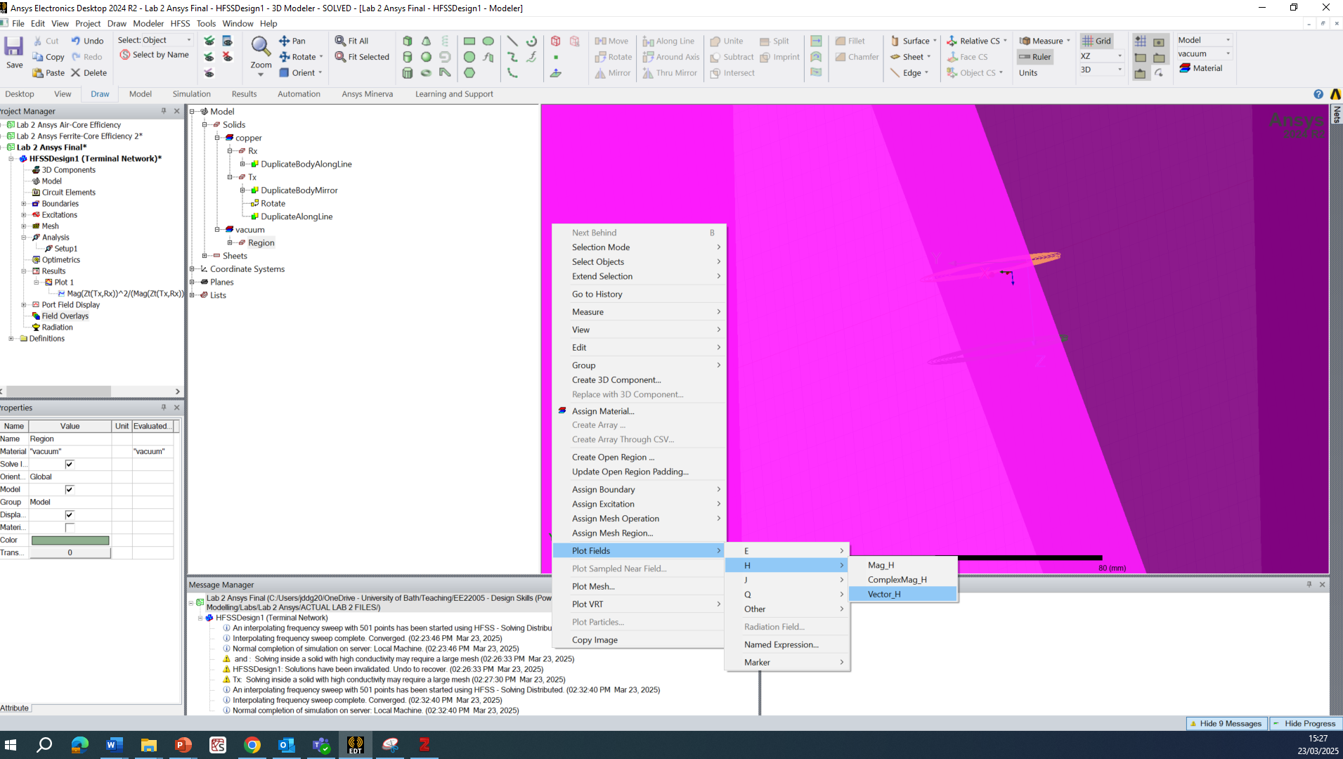
Make sure to select In Volume AllObjects and click Done:

Initially this may look very unclear, so we need to change the plot settings to something like those below (feel free to play around with these):

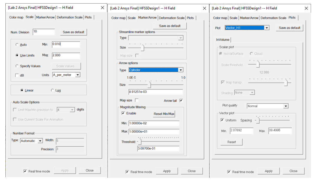
Which should produce a nice plot of the magnetic field:

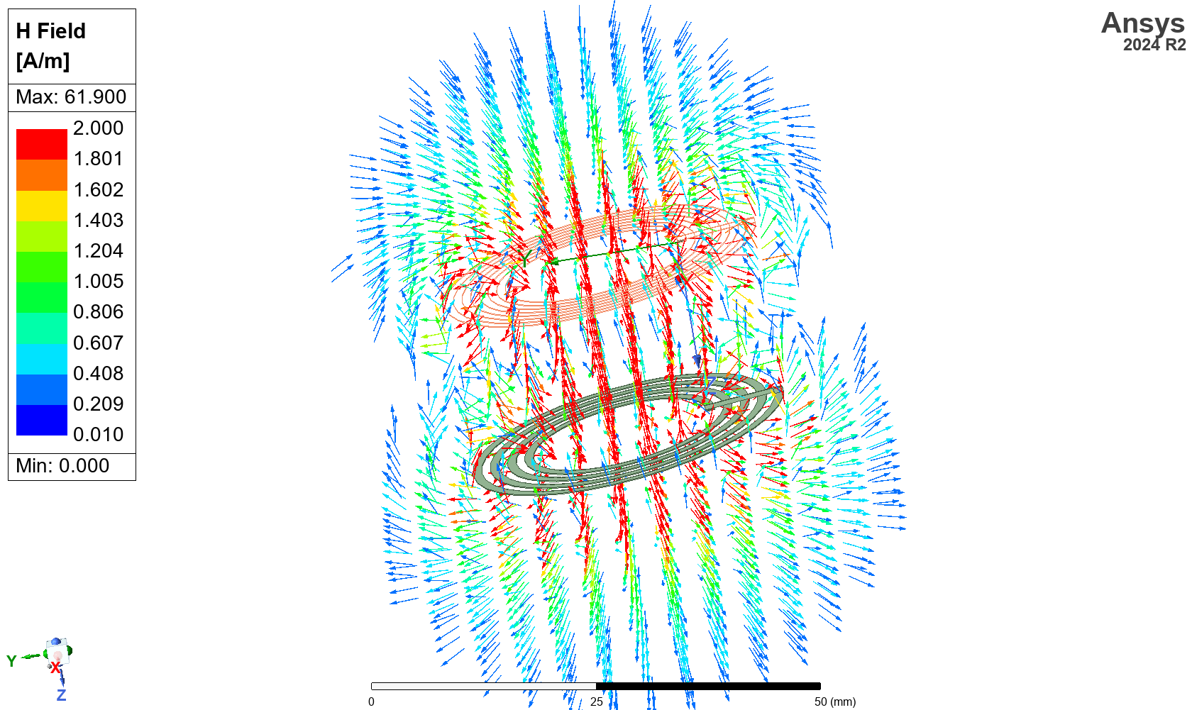
We can animate this (evaluate at different phases) by right-clicking and selecting Animate:

Here ends Section 1 required for Knowledge level.

Section 2: Ferromagnetically Cored WPT System (A)

To claim the skill at Application level, you can extend the simulation from Section 1 by considering what happens if design one or both coils using ferromagnetic material.

In general, we use ferromagnetic materials (iron, ferrite) to shape, suppress or reinforce the magnetic fields as illustrated in .

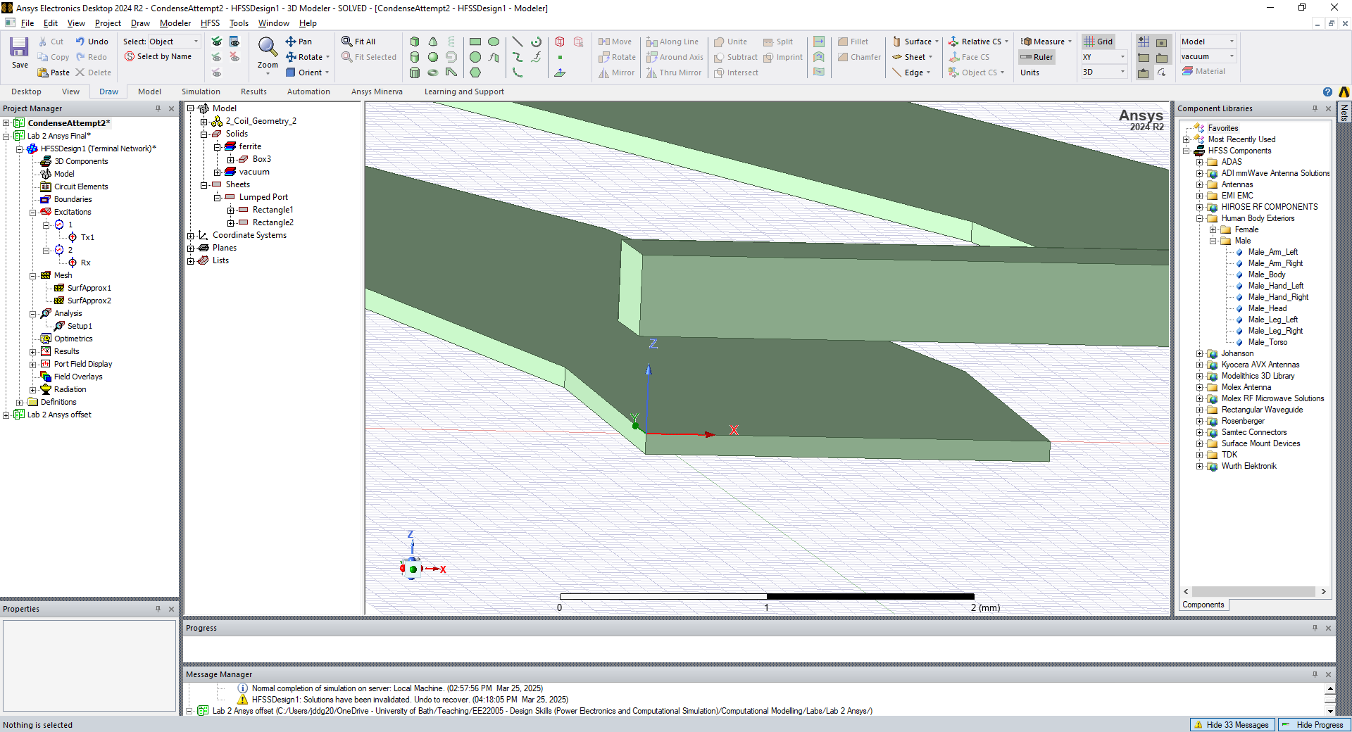
Try adding some ferrite (which is in the standard materials library) to make one of your coils ferromagnetically cored. Or you could put some ferrite between the two coils and see what happens. Some questions you might like to address for claiming the skill at Application level include:

• Does the inductance (and therefore impedance, Z) increase or decrease when ferrite is added?
• Does the mutual coupling increase or decrease?
• Does the power transfer efficiency increase?
• What does the field distribution in space look like?
• Are there any losses in the ferrite?
• How does the simulator account for these losses?
• What if I put my hand in between the coils?
• What if I increase the maximum frequency of the simulation?

[1] M. Maaß, A. Griessner, V. Steixner, and C. Zierhofer, ‘Reduction of eddy current losses in inductive transmission systems with ferrite sheets’, Biomed. Eng. OnLine, vol. 16, no. 1, p. 3, Jan. 2017, doi: 10.1186/s12938-016-0297-4.