1D Heat Equation in Python
In this lab we will simulate heat transfer in one dimension in Python.
In Section 1, we will go step-by-step through the simulation of a one-dimensional rod with an initial sinusoidal temperature distribution using an explicit time stepping method.
Initially, we will have a Dirichlet boundary conditions and see heat dissipate through the ends of the rod. We will then change to Neumann boundary conditions to simulate insulated ends to observe heat disperse through the rod. Most of the code will be provided, with a few key lines removed. The work in Section 1 can be used to claim the associated skill at Knowledge level.
In Section 2, we will look to solve the same setup using an implicit solving method. Some of the structure of how to do this will be set up for you, but key bits of code will be left for you to complete. The work in Section 2 can be used to claim the associated skill at Application level.
Section 1: Explicit Solver for 1D Heat Equation (K)
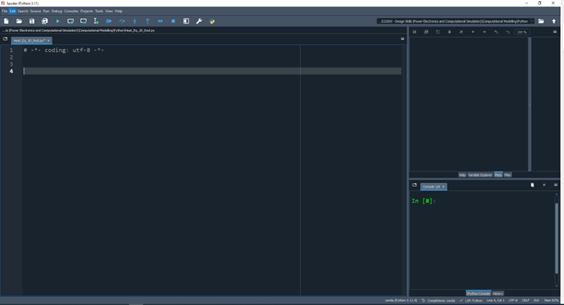
Open a new Python script in the IDE of your choice. Here we will be using Spyder as seen in . Ensure that you save the script with a recognisable name e.g. Heat_Eq_1D_Rod.py and save it regularly to avoid losing your work.
Step 1: Import Packages
First, we need to import a few Python packages, including for plotting and animation of our simulations:
  import numpy as np
  import matplotlib.pyplot as plt
  from matplotlib.animation import FuncAnimation, PillowWriter
  import os
import timeStep 2: Initialise Simulation Parameters
Next, we want to initialise the parameters for our simulation, we want to simulate the behaviour of a 1m long rod with $\alpha$ thermal diffusivity of 0.05 $m^2/s$. We want to run this simulation over 5 seconds. To discretise the rod is space, we will split it up into 100 spatial points.
#---------------------------------------------------------------------------
# Physical and computational parameters
#---------------------------------------------------------------------------
L = 1.0           # Length of the rod (meters)
T = 5             # Total simulation time (seconds)
N = 100           # Number of spatial grid points
M = 12         	# Number of time steps
alpha = 0.05      # Thermal diffusivity coefficient of material (m²/s)
dx = L / N        # Spatial step size (meters)
dt = T / M # Time step size (seconds)Step 3: Check for stability
As we are using an explicit method, we need to check whether the solver is stable using the stability criterion for diffusion:
\[\begin{equation} \label{eq:exampleEquation} \begin{split} r= \frac{\alpha\Delta t}{\Delta x^2} ≤ 1/2 \end{split} \end{equation}\]r = XXXXXXXXXXX
INSERT EXPRESSION FOR r (STABILITY CRITERIA)
AND CHANGE TIMESTEP TO ENSURE STABILITY (SEE LECTURE 3)
assert r <= 0.5, "Stability condition violated! Decrease dt or increase dx."Step 4: Initialise Computational Domain
We need to set up some arrays to handle our variables as they evolve in time and space. We will first make our spatial grid according to the parameters we setup earlier by using a 1D array:
# Create spatial grid
x = np.linspace(0, L, N+1) # Equally spaced points from 0 to LWe also want to initialise our temperature array over both time and space. As we have both time and a single spatial dimension, we will use a 2D array:
# Create temperature array: u[time_step, position]
u = np.zeros((M+1, N+1)) # M+1 time steps, N+1 spatial pointsStep 5: Set Rod Initial Conditions
We need to specific the starting temperature distribution in the rod. We will say that we start at t=0 with a sinusoidal temperature distribution with an amplitude of 50°C and an offset of 20°C.
# Set initial conditions for rod temperature distribution
u[0, :] = np.sin(np.pi * x / L) * 50 + 20 # Temperatures from 20°C to 70°Step 6: Set Boundary Conditions
We need to specify to the solver how the solver should behave as it hits the edge of our domain of interest i.e. the two ends of the rods. To start off, we want to simulate what happens when the temperatures at both the ends of the rods are fixed. This simulates that they are effectively heat-sunk. To do this we will use Dirichlet boundaries where we directly specify the value of the dependent variable at the boundary:
# Time-stepping loop
for n in range(M):  # Loop through time steps
    # Apply Dirichlet boundary conditions (fixed temperature at boundaries)
    u[n+1, 0] = 20     # Left boundary fixed at 20°C
XXXXXXXXXX INSERT EXPRESSION FOR RIGHT BOUNDARY CONDITION (FIXED 20°C)Step 7: Set up the solver using the Finite Difference method with Explicit time-stepping
We now want to set up our solver to step through both time and space to simulate how our system will evolve based on the initial conditions, scenario and the underlying physics
#------------------------------------------------------------------------------
# Numerical solution using Finite Difference Method (Explicit scheme)
#------------------------------------------------------------------------------
# Time-stepping loop
for n in range(M):  # Loop through time steps
    # Apply Dirichlet boundary conditions (fixed temperature at boundaries)
    u[n+1, 0] = 20     # Left boundary fixed at 20°C
    XXXXXXXXXX INSERT EXPRESSION FOR RIGHT BOUNDARY CONDITION (FIXED 20°C)


    # Update interior points using the finite difference approximation
    for i in range(1, N):  # Loop through interior spatial points
XXXXXXXXXX INSERT EXPRESSION FOR EXPLICIT UPDATE EQUATION Step 8: Visualise Results
We now want to be able to see how the temperature in our rod evolves over time. We can do this most easily with animations. Note that we don’t want to see the result at every timestep that we calculate as this would take too long to create, so we specify a maximum of 200 frames.
The first animation uses an xy line graph evolving over time and the second uses a colour-coded heatmap. We will save these animations as .gif files in our current directory. Some example code (Windows only) is below – feel free to copy this code directly or use your own method to visualise the results:
#------------------------------------------------------------------------------
# Visualization 1: 1D Line Plot Animation
#------------------------------------------------------------------------------

# Clear everything before starting -----
plt.close('all')  # Close all existing figures

# Create figure and axis for the line plot
fig1 = plt.figure(figsize=(10, 6))
ax1 = plt.gca()

# Create initial line
line, = ax1.plot(x, u[0, :])
time_text1 = ax1.text(0.02, 0.95, '', transform=ax1.transAxes)

# Set up the plot
ax1.set_xlim(0, L)
ax1.set_ylim(0, 80)
ax1.set_xlabel('Position (m)')
ax1.set_ylabel('Temperature (°C)')
ax1.set_title('Heat Equation Solution with Dirichlet Boundaries (1D Rod)')
ax1.grid(True)

# Animation update function for line plot
def update_line(frame):
    n = frame * (M // 200)  # Show 200 frames total
    line.set_ydata(u[n, :])
    time_text1.set_text(f't = {n*dt:.2f} s')
    return line, time_text1

# Create the line plot animation
anim1 = FuncAnimation(
    fig1,
    update_line,
    frames=200,
    interval=50,
    blit=True,
    repeat=True
)

# Save the line plot animation
if os.path.exists('heat_equation.gif'):
    try:
        os.remove('heat_equation.gif')
    except Exception as e:
        print(f"Warning: Could not remove existing heat_equation.gif file: {e}")

writer1 = PillowWriter(fps=20)
anim1.save('heat_equation.gif', writer=writer1)

#------------------------------------------------------------------------------
# Visualization 2: 2D Heatmap Animation
#------------------------------------------------------------------------------
# Create figure and axis with larger size for better visualization
fig2, ax2 = plt.subplots(figsize=(12, 4))

# Create a 2D representation of the rod by replicating the 1D temperature array
rod_thickness = 20  # Visual thickness of the rod (pixels)
rod_2d = np.tile(u[0, :], (rod_thickness, 1))  # Copy the 1D array vertically

# Create the image object for visualization
im = ax2.imshow(rod_2d,
               aspect='auto',               # Adjust aspect ratio automatically
               extent=[0, L, -0.1, 0.1],    # Set the display limits [xmin, xmax, ymin, ymax]
               cmap='inferno',              # Use inferno colormap (good for temperature)
               vmin=20, vmax=70)            # Fix color scale to temperature range

# Add colorbar to show temperature scale
cbar = plt.colorbar(im)
cbar.set_label('Temperature (°C)', size=14)

# Set labels and title for the plot
ax2.set_xlabel('Position (m)', size=14)
ax2.set_title('Heat Equation Solution: Temperature Distribution in Rod', size=16, pad=20)

# Remove y-axis ticks as they're not meaningful for this visualization
ax2.set_yticks([])

# Add text to display current simulation time
time_text2 = ax2.text(0.02, 0.95, '', transform=ax2.transAxes, fontsize=12, color='white')

# Animation update function for heatmap
def update_heatmap(frame):
    # Select time steps to visualize (we don't need to show all 10,000 steps)
    n = frame * (M // 200)  # Sample 200 frames from the full simulation

    # Update the 2D rod representation with current temperature profile
    rod_2d = np.tile(u[n, :], (rod_thickness, 1))
    im.set_array(rod_2d)

    # Update the time display
    time_text2.set_text(f't = {n*dt:.2f} s')

    # Return the objects that have been modified (required for blit=True)
    return im, time_text2

# Create the heatmap animation with 200 frames
anim2 = FuncAnimation(
    fig2,                # Figure to animate
    update_heatmap,      # Update function
    frames=200,          # Number of frames to display
    interval=50,         # Delay between frames in milliseconds
    blit=True,           # Use blitting for efficiency
    repeat=True          # Loop the animation
)

# Save the heatmap animation
if os.path.exists('heat_equation_rod.gif'):
    try:
        os.remove('heat_equation_rod.gif')
    except Exception as e:
        print(f"Warning: Could not remove existing heat_equation_rod.gif file: {e}")

writer2 = PillowWriter(fps=20)  # 20 frames per second
anim2.save('heat_equation_rod.gif', writer=writer2, dpi=150)  # Save with 150 dpi resolution

# Check if files exist and have content
if os.path.exists('heat_equation.gif') and os.path.getsize('heat_equation.gif') > 0:
    os.startfile('heat_equation.gif')  # Windows-specific command
else:
    print("Error: heat_equation.gif not found or empty")

# Small delay before opening second file to prevent overlap
time.sleep(0.5)

if os.path.exists('heat_equation_rod.gif') and os.path.getsize('heat_equation_rod.gif') > 0:
    os.startfile('heat_equation_rod.gif')  # Windows-specific command
else:
    print("Error: heat_equation_rod.gif not found or empty")

print("Animation files should now be open in your default GIF viewer")If successfully implemented, the outputs should look like the images in and below:

Step 9: Change to Insulating Boundary Conditions
We now want to simulate the behaviour of the rod assuming that the ends of the rod are perfectly insulating (i.e. no heat can escape). To do this we need to specify insulating, or von Neumann, boundary conditions. The key here is to recognise that the temperature gradient (∂u/∂x) at the boundary will be zero.
# Time-stepping loop
for n in range(M):  # Loop through time steps
    # Apply Neumann boundary conditions (insulating/zero heat flux at boundaries)
    # For zero heat flux: ∂u/∂x = 0 at x = 0 and x = L
    # Using second-order accurate one-sided difference:
    # For left boundary (x = 0): u_0 = u_1
    # For right boundary (x = L): u_N = u_{N-1}
    u[n+1, 0] = u[n+1, 1]     # Left boundary (insulating)
XXXXXXXXXXXX INSERT EXPRESSION FOR RIGHT NEUMANN BOUNDARY CONDITION If successfully implemented, you should now get outputs that look like and below:
Here ends Section 1 which you can claim for Knowledge.
Implicit Solver for Heat Equation in 1D (A)
As we mentioned in Lecture 2, we can solve PDEs numerically using explicit or implicit methods. We said that explicit methods can be unstable, which we will have seen in Section 1 where we need to satisfy the von Neumann stability criteria. Using implicit time stepping on the other hand, we are guaranteed stability but have to solve each timestep iteratively.
To do this, we will produce code that is similar to that using the explicit method. All parameters, initial conditions, boundary conditions will be the same, however, we will change the ‘Solver’ section to implement an implicit scheme. There are several different options for this, but we could use the Jacobi method covered briefly in Lecture 2:
#------------------------------------------------------------------------------
# Numerical solution using Finite Difference Method (Implicit scheme)
#------------------------------------------------------------------------------
# Time-stepping loop (keep other code same/similar to explicit scheme)

# Jacobi iteration parameters
tol = XXXXXXXXX CHOOSE CONVERGENCE TOLERANCE (A SMALL NUMBER)
max_iter = XXXXXXXXX CHOOSE MAX ITERATIONS FOR CONVERGENCE

for n in range(M):
    # Apply boundary conditions (your choice of Dirichlet or Neumann)
    XXXXXXXXX INSERT EXPRESSION FOR BOUNDARY CONDITIONS

    # Initialize the solution for the current time step with previous values
    u[n+1, 1:N] = u[n, 1:N]

    # Create temporary arrays for Jacobi iteration
    u_old = np.copy(u[n+1, :])
    u_new = np.copy(u[n+1, :])

    # Iterative solution using Jacobi method
    for iter in range(max_iter):
        # Update interior points
        for i in range(1, N):
            XXXXXXXXXXXX INSERT IMPLICIT UPDATE EQUATION

        # Check convergence
        error = np.max(np.abs(u_new - u_old))
        if error < tol:
            break

        # Update old solution for next iteration
        u_old = np.copy(u_new)

    # Update solution for current time step
    u[n+1, :] = u_new[:]

    # Print progress periodically
    if n % 100 == 0:
print(f"Time step {n}/{M} completed ({n/M*100:.1f}%)")Discussion and Reflection
Now that you have ‘simulations’ of the 1D heat equation for a rod using both explicit and implicit methods, it is time to think about how to use these and what to look out for when building simulations.
Remember, for Application level for this skill, you should reflect on some aspect of the simulation and why you might use one method or simulation parameter over another.
Possible questions you may answer include:
- What is the minimum timestep for explicit vs implicit methods?
- Does explicit or implicit require more compute?
- What is the physical meaning of the two different boundary conditions we have seen and where might I apply them when working on electronics?
- How might I discretise the rod in space differently?
- How would I define boundaries for electromagnetic fields?
- What is the best way to visualise my results?
- If I pick up the rod at time of 2.3 seconds at position 0.34 m from one end, would I burn my hand? Does it depend on the boundary conditions?
- What level of accuracy is sufficient?
- Can I set up a simulation that my computer can’t solve?
- Can I set up a simulation that a supercomputer couldn’t solve in a million years?