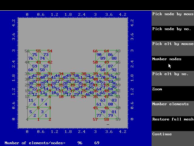
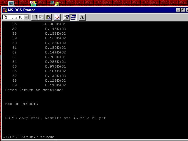
The pre-processor has produced a new data file, h2.dat, containing the details of the mesh shown above. We now perform the main finite element analysis, by compiling the source code poiss.for into poiss.exe (using whichever Fortran compiler is available, as the program only uses standard Fortran77), and running it with h2.dat as the input file. The results - the values of the unknown variable u at each of the 96 nodes - are listed on the screen. In order to see these results graphically, we run the post-processor FELVUE by issuing the command "run77 felvue"...
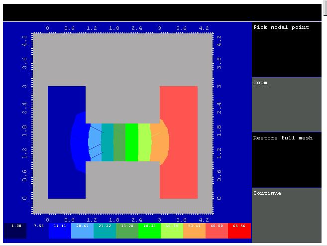
The post-processor gives a coloured contour plot of the results. In this example, the Dirichlet boundary values have been set at U=1.0 on the vertical plane x=0, and U=60.0 on the plane x=4.0.
The following plot was produced without defining in PREFEL the Dirichlet boundary values; in this
case, the POISS program uses an inbuilt boundary function. When supplied, this is
bdrfn(x,y) = x*x - y*y
but this can of course be changed in the source code and recompiled.
The picture can be zoomed; the zoom area is
defined by clicking on two opposite corners...
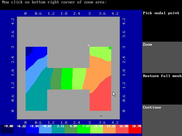
Here, the white cross shows the top left corner of the zoom area chosen, and the mouse is about to click on the bottom right corner. The zoom plot of the area defined, is shown below...
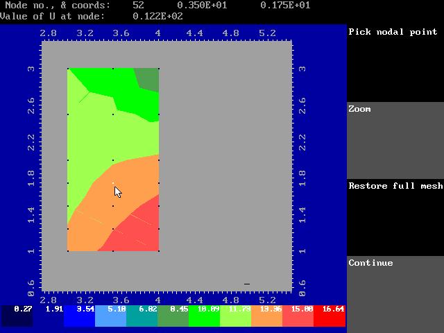
In the picture above (from the old MS-DOS version), the user has picked a particular nodal point: its node number, coordinates and nodal value of u are then displayed in the dialogue box at the top of the screen.
The two methods of defining Dirichlet boundary values can be combined; any Dirichlet nodes not defined by the planes data, will use the boundary function. In the following result, the left-hand Dirichlet boundary was set at U=1.0, while the linearly-varying boundary function was used on the right-hand boundary.
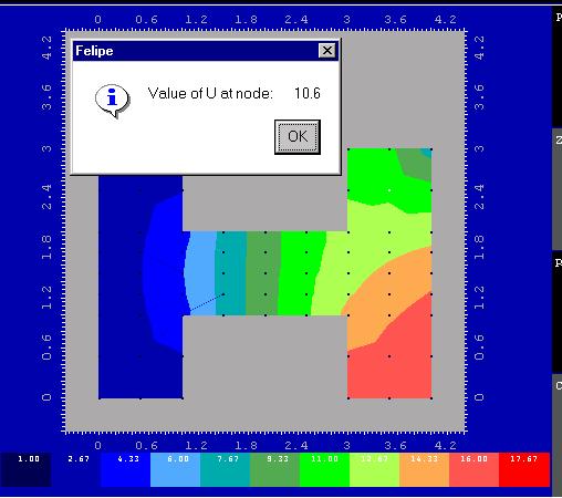
In the new Win32 version, when the user picks a nodal point with the mouse, pop-up windows show first its coordinates, and then its nodal value (as illustrated above).