Finite Impulse Response Filter Design

Skills Mapping

Dr J. G-H-Cater - 21/01/2025

Skills ? :

The Limits of Filtering Signals in the Real World

This lab explores the design and implementation of practical Finite Impulse Response (FIR) filters using MATLAB. FIR filters are widely used in digital signal processing applications due to their inherent stability and linear-phase characteristics. However, ideal FIR filters require infinite non-causal coefficients, which is not practical in real life. Through this hands-on experience, you will gain a deeper understanding of FIR filter design principles, and practice the art of windowing as a method to produce practical filters to a specification.

FIR Filter design is a complex topic, and this lab is therefore written to guide the reader through the whole process. To that end, successful completion of this lab should support a ‘Knowledge’ level claim against the Finite Impulse Response Design skill.

You will require a pen and paper while performing this lab to make notes and derive equations. It is recommended that you physically record your answers for each exercise to avoid loss of work if the Lab PCs crash. You will also require a copy of MATLAB (version R2023b or later).

Lab Summary

In this lab, you will be provided with a recorded signal that requires filtering. A provided tool will allow you to verify your answers as you go. Once finished, this same tool may be used to generate two documents that contain all required elements for claiming the FIR design skill on Mahara, making for a simple upload process.

You are encouraged to complete this lab individually if possible, as that will yield the best learning outcomes. The tool will provide each student with a unique signal to process, meaning that you will have different answers from others during the lab. Your university username is used to generate your signal, and verify your answers during marking, so it is essential to enter it correctly when using the tool.

Working in pairs: Since the tool accepts only one username, pairs must decide which username to use, and then both stick to using that one username throughout the lab. While the generated documents will only display the chosen username, both students may still upload them to claim the skill. In such cases, both partners must add a text block to the Mahara page that states they were working in a pair and includes the name and username of their group partner.

The Signal

The signal in question is an Amplitude Modulated (AM) signal, which encodes data (1’s and 0’s) by modifying the amplitude of a higher frequency carrier. While you do not need to understand the principles behind AM signals to complete this lab, an example of such a signal may be seen in .

The AM signal with the amplitude clearly changing once every second.

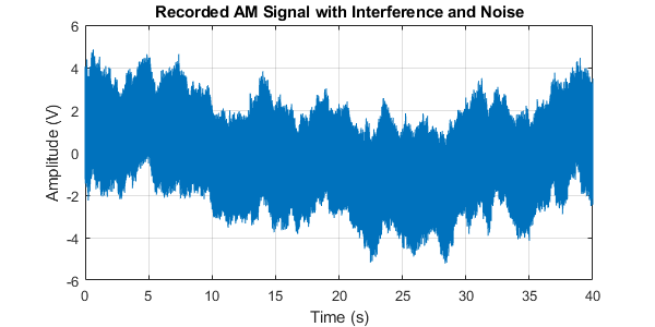
Sadly, as is often the case when working with real data, your signal has been corrupted by both noise and interference - resulting in a recording similar to the one shown in .

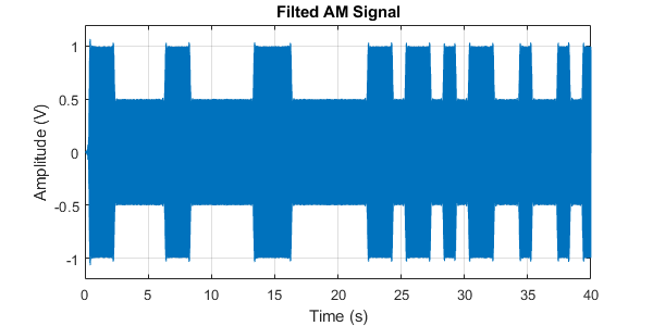
The recorded AM signal contains noise and interference making it barely recognizable.

It will be your task to design a filter to extract the original data from this noisy signal. If successful you should find that plotting your filters output will look similar to (but not exactly like) the noise free AM signal above - as shown in .

The filtered AM signal looks more like the original, however there are still some imperfections as a result of filtering process. Filters must be designed to achieve a good balance between filter complexity and the resulting imperfections in the output.

Setup

As stated in the lab summary, a MATLAB program is provided that may be used to generate the signal, check answers, and generate documents for uploading to Mahara. In this section, we will get set-up for the lab by downloading and running the tool.

Directory and Tool Setup

First create a new folder for this project that will be used to contain all the files related to this lab.
Open MATLAB and navigate to the folder you created in step 1.
Download the FIRSkillTool.p file using the button below and move it into this folder. Make sure not to change the name of this file.

Download FIR Skill Tool

You should now see the FIRSkillTool.p file listed in MATLAB in the current folder browser on the left.

You can run this tool by either typing ‘FIRSkillTool’ in the command window or right-clicking on the file in the MATLAB folder browser and selecting ‘Run’.

If successful, you should find that a new window opens, as shown in .

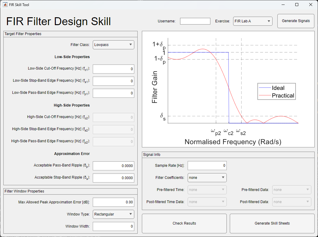
The FIR Filter Design Skill tool may be used to generate signals, verify answers, and generate skill sheets used to claim the skill on Mahara.

You may notice that there is an Exercise dropdown at the top right of this tool. If you wish to use the skill sheet generator to claim FIR Filter Design at application or synthesis level, then you do so by setting the exercise to ‘Custom’. This will disable the results checking and signal generation - but allows you to enter the filter criteria and signals required to claim the skill.

Generating the Signal

Enter your username (see the warning at the top of this lab script if working in a pair) into the username box.
Set the exercise to ‘FIR Lab A’.
Click the ‘Generate Signals’ button.

Checking your MATLAB workspace, you should see that two signals have been created LabA_Time and LabA_Signal. The former is the time at each sample, while the latter is the amplitude of the signal at each sampled moment.

Plot the signal against time and check that it is of a similar form (but distinct) to that shown in .

Extracting Signal Properties

Before a filter can be created to restore the original AM signal, it is critical to first identify the properties of the signal. This includes the sample rate, frequencies that make up the desired signal, the frequencies of any interference, and a general idea of the noise level.

Interference and noise are both unwanted signals that can degrade the quality of a desired signal, but they originate from different sources and have distinct characteristics.

Interference

Interference refers to unwanted signals that originate from external sources, often other communication systems or electronic devices operating in a similar frequency range. It is typically predictable and can sometimes be mitigated through filtering or frequency separation.

Examples of interference:

Radio frequency interference (RFI) from nearby electronic devices.
Crosstalk between adjacent communication channels.
Electromagnetic interference (EMI) from power lines or industrial equipment.
Intentional interference, such as jamming signals in wireless communications.

Key characteristics:

Often caused by identifiable sources.
Can be periodic, continuous, or somewhat deterministic behavior.
Usually mitigated using shielding, filtering, and/or careful frequency regulation and management.

Noise

Noise refers to random, unpredictable disturbances that are inherent in the system or environment. It is typically caused by natural processes and cannot be completely eliminated, though it can sometimes be reduced.

Examples of noise:

Thermal noise (due to random motion of electrons).
Shot noise (due to discrete nature of electrical charge).
Atmospheric noise (caused by natural sources like lightning).
Quantum noise (in extremely sensitive systems).

Key characteristics:

Random, and unpredictable.
Often follows a statistical distribution (e.g., Gaussian noise, white noise, or red noise).
Can be reduced but not entirely eliminated by good shielding and grounding.

In this scenario, the signal’s properties are unknown and must be determined through direct analysis of the signal using the techniques introduced in the signal processing lectures. This includes both time-domain analysis (e.g., plotting the signal and examining the raw data) and frequency-domain analysis (e.g., computing and visualizing the FFT of the signal). While tools like spectrograms are often used for analyzing unknown signals, this lab has been designed to make this unnecessary, streamlining the process and eliminating the need for such tools on this occasion.

Given that provided signals included a time signal, it is possible to calculate the sample rate by analyzing the difference in time between two adjacent samples ($T_s$). From this information you can calculate the sample rate, or frequency, using $F_s = 1/T_s$.

Now that the sample rate is known, it is possible to perform frequency-domain analysis on the signal. For this we will use MATLABs fft() function.

While very powerful, the output from the MATLAB FFT function requires some treatment to produce physically meaningful measures. This is discussed in the MATLAB fft documentation and it is strongly encouraged that you read the documentation and work through the ‘Noisy Signal’ example before continuing.

FFT Analysis Tools

Based on examples provided in the MATLAB MATLAB fft documentation, create a function named plotFFT(sampleRate, signal) that takes a sample rate and signal as input arguments and generates a Single-Sided Amplitude Spectrum Plot.

Create a second function named plotLogFFT(sampleRate, signal) that performs the same operations as previously, but instead of using plot() to plot the fft, use loglog() to create a plot that has logarithmic scale on both the x- and y-axis.

Beyond this lab, these functions will be useful for analyzing other signals in the future, and having them available will therefore save time when working on any other signal processing tasks. Building out a toolkit of common techniques and tools in this manner is a sensible approach for any engineer.

To verify that the plotFFT() function works correctly, simply generate a test signal, such as y = cos(2*pi*F*LabA_Time), where F is a known frequency below the Nyquist limit. Separately apply the plotFFT() and plotLogFFT() functions to this signal, confirming that the resulting spectrums correctly display a single peak at the expected frequency.

Identifying Noise

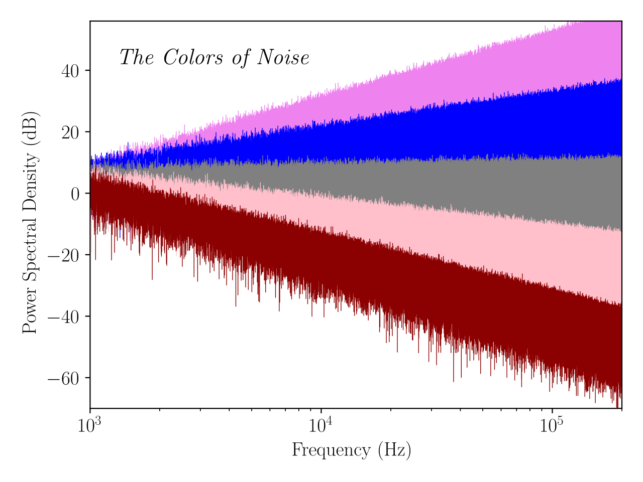
Noise in inherently random - however the power spectral density can follow patterns, resulting in what are referred to as different colors of noise. Probably the most commonly used type of noise is ‘white noise’ which has a flat power spectra when plotted in dB. Other common types of noise also form a slope when plotted on a log-log graph, with the angle of the line telling you what type of noise might be present.

Noise can come in many 'colors', shown here (from top to bottom) is Violet, Blue, White, Pink, and Brown/Red. The power spectral densities are arbitrarily normalized such that the value of the spectra are approximately equivalent near 1 kHz.

Using the plotLogFFT() function, graph the unknown LabA_Signal and identify what type of noise may be present - don’t worry about calculating the exact slope or identifying a specific color, instead identify the general trend or direction of the noise.

With this information in mind, look for regions where the signal diverges from the noise floor and make a note of the approximate frequency range where this occurs.

Identifying Signals and Interference

With the noise loosely identified, the AM signal and any other interference signals may now be found. For this lab, you may assume that any interference signals will be single tones, meaning they will show up as a single and narrow spike in the FFT. In contrast the AM signal will have a large spike that appears to ‘pinch’ up around it’s base, where the modulation has spread power into surrounding frequencies.

Using the plotFFT() function, graph the unknown LabA_Signal and zoom into the x-axis region where signals were showing on the logarithmic spectrum plot.

Given that this signal has a single AM modulated waveform, and two interference tones, try to identify and make note of the central frequency for each. Note the type of spike can be identified by looking at the shape in the surrounding frequencies, while the central frequency for each may be found by using the DataTips tool in the plot window and placing a DataTip at the highest point of each of the three spikes.

Defining a Filter

We have now identified the noise, two interference tones, and the AM carrier frequency (or central frequency) within the signal. With this information we can now specify a filter to remove the interference and noise without changing the AM waveform.

Based on the position of the AM waveform and the two interference tones, decide whether the filter must be a low-pass, high-pass or band-pass filter. You can enter this into the Filter Class box on the FIR Skill Tool to verify your answer for this lab.

Defining the Ideal Filter

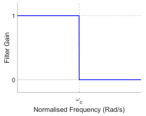
In the ideal case, a filter would be able to selectively allow a desired range of frequencies through unmodified, while fully removing the undesired frequencies. For example, the frequency response of an ideal low-pass filter, $H_i(e^j\omega)$, would look like a step function with it’s falling edge located at the cut-off frequency, $\omega_c$.

A plot of an ideal low-pass filter frequency response, showing an output of magnitude 1 for all frequencies below the cut-off frequency and a magnitude of 0 for all frequencies above the cut-off frequency. — The frequency response for an ideal low-pass filter, showing the cut-off frequency located at $\omega_c$.

Mathematically, the frequency response may be defined as:

\[\begin{equation} H_{LP}(e^{j\omega})=\left\{ \begin{array}{ll} 1, & \mbox{if $\left|\omega\right| < \omega_c$}.\\ 0, & \mbox{otherwise}. \end{array} \right. \end{equation}\]

Given that the frequency response describes the filter in the frequency domain, a time-domain impulse response for this ideal filter may be found by applying the inverse Fourier transform. It is worth noting that the inverse Fourier operation, described in Equation \eqref{eq:InverseFourier}, contains an integration from $-\pi$ to $\pi$. This is because the normalized frequency-response of any filter will always sit within this range, with the values mirrored about the y-axis.

\[\begin{align} h_{LP}[n] &= \frac{1}{2\pi}\int^\pi_{-\pi}{H(e^{j\omega})e^{j\omega n}.d\omega} \label{eq:InverseFourier} \\ &= \frac{1}{2\pi}\int^{\omega_c}_{-\omega_c}{e^{j\omega n}.d\omega} \nonumber \\ &= \frac{1}{2\pi}\left[\frac{1}{jn}e^{j\omega n}\right]^{\omega_c}_{-\omega_c} \nonumber \\ &= \frac{1}{\pi n}\left[\frac{1}{2j}\left(e^{j\omega_c n}-e^{-j\omega_c n}\right)\right] \nonumber \\ &= \frac{1}{\pi n}\sin(\omega_c n) \label{eq:IdealTimeSin} \end{align}\]

Looking closely, it may be seen that equation \eqref{eq:IdealTimeSin} has a discontinuity at $n=0$. To remove this, we can convert the equation into another form using the relationship $\text{sinc}(x)=\sin(\pi x)/\pi x$ and multiplying $h_{LP}$ by ${\omega_c n}/{\omega_c n}$. This yields:

\[\begin{align} h_{LP}[n] &= \frac{1}{\pi n}\cdot\frac{\omega_c n}{\omega_c n}\sin(\omega_c n) \nonumber \\ &= \frac{\omega_c}{\pi}\cdot\frac{\sin(\omega_c n)}{\omega_c n} \nonumber \\ &= \frac{\omega_c}{\pi}\text{sinc}\left(\frac{\omega_c n}{\pi}\right) \label{eq:DiscreteIdealTime} \end{align}\]

For FIR filters of any kind, it may be shown that the coefficients are given by the unit-impulse response of the filter. Therefore, with Equation \eqref{eq:DiscreteIdealTime} we now have a way to define the coefficients for our generalized ideal low-pass filter.

A plot showing examples of values produced by Equation 12 to create an ideal low-pass filter. — A plot showing some of the coefficients required to create the ideal low-pass filter.

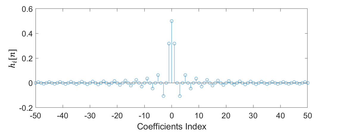
There is one major issue, however, as the impulse response in is both infinite in length ($n \in \mathbb{Z}$) and non-causal (uses both positive and negative indexed coefficients). These two properties meaning that it is impossible to build a practical filter with this maths alone.

Ideal Band-Pass Filters Challenge

The above example derives an equation to define the infinite coefficients required to implement an ideal low-pass filter. Given that the frequency response of a generic ideal band-pass filter may be defined as:

\[\begin{equation} H_{BP}(e^{j\omega})=\left\{ \begin{array}{ll} 1, & \mbox{if $\omega_{c1} \leq \left|\omega\right| \leq \omega_{c2}$}.\\ 0, & \mbox{otherwise}. \end{array} \nonumber \right. \end{equation}\]

Use the inverse Fourier equation shown in Equation \eqref{eq:InverseFourier} to define an expression for the discrete time-domain impulse response (and therefore the coefficients) of a generic ideal band-pass filter. Keep an eye out for the $sinc()$ function again - as it will show up a couple of times.

It may be good to reflect on how this relates to the definition of the low pass filter, and why this relationship may exist.

Don't forget to account for the fact that normalized frequency is defined between $-\pi$ and $\pi$, so both the positive and negative regions of the frequency domain must be considered when integrating.

Solution

Applying the same methods as with the low-pass filter yields:

\[\begin{align} h_{BP}[n] &= \frac{1}{2\pi}\int^{\pi}_{-\pi}{H(e^{j\omega})e^{j\omega n}.d\omega} \nonumber \\ &= \frac{1}{2\pi}\left[\int^{\omega_{c2}}_{\omega_{c1}}{e^{j\omega n}.d\omega} + \int^{-\omega_{c1}}_{-\omega_{c2}}{e^{j\omega n}.d\omega}\right] \text{ by piecewise.}\nonumber \\ &= \frac{1}{2\pi}\left[\left[\frac{1}{jn}e^{j\omega n}\right]^{\omega_{c2}}_{\omega_{c1}} + \left[\frac{1}{jn}e^{j\omega n}\right]^{-\omega_{c1}}_{-\omega_{c2}}\right] \nonumber \\ &= \frac{1}{2\pi}\left[\frac{1}{jn}\left(e^{j\omega_{c2} n}-e^{j\omega_{c1} n} + e^{-j\omega_{c1} n}-e^{-j\omega_{c2} n}\right)\right] \nonumber \\ &= \frac{1}{\pi n}\left[\frac{1}{2j}\left(e^{j\omega_{c2} n}-e^{-j\omega_{c2} n}\right) - \frac{1}{2j}\left(e^{j\omega_{c1} n}-e^{-j\omega_{c1} n}\right)\right] \nonumber \\ &= \frac{1}{\pi n}\sin\left(\omega_{c2} n\right) - \frac{1}{\pi n}\sin\left(\omega_{c1} n\right) \text{ by inverse Euler} \nonumber \\ &= \frac{\omega_{c2}}{\pi}\text{sinc}\left(\frac{\omega_{c2} n}{\pi}\right) - \frac{\omega_{c1}}{\pi}\text{sinc}\left(\frac{\omega_{c1} n}{\pi}\right) \nonumber \end{align}\]

The ideal band-pass FIR filter can be thought of as the difference between two low-pass filters, each with a specific cutoff frequency. The second, with a lower cut-off frequency, is subtracted from the first, with a higher cut-off frequency. Effectively this means that the first low-pass filter has removed all signals with frequency above $\omega_{c2}$, while the second contains only signals with frequency below $\omega_{c1}$. Subtracting the second result from the first result yields only the signals with frequencies between $\omega_{c1}$ and $\omega_{c2}$ (i.e. those in the first output that were not also present in the second).

In other words:

\[\begin{equation} h_{BP}[n] = h_{LP,\omega_{c2}}[n] - h_{LP,\omega_{c1}}[n] \end{equation}\]

Specifying Practical Filter Properties

Since implementing the ideal filter coefficients is not physically possible, some compromise must be made - resulting in a filter which only somewhat approximates the desired filter frequency response. The infinite coefficients that make up the ideal filter must be shortened to a finite set of coefficients that still achieve comparable results. As the number of coefficients is reduced from the ideal infinite set, the shortened filter will form a decreasingly accurate approximation of the ideal filter. To ensure that the final result is still useful, the frequency response of this approximated filter must not differ from the ideal filter frequency response by too much. To this end, filter specifications can be used to define what level of approximation is acceptable without negatively impacting the final solution. Careful design of these specifications will also help ensure that the final solution isn’t over-designed, without compromising too much on the final signal quality.

Typical filter specifications include a range of properties that depend on both the type of filter and the end application. The following are properties are useful metrics by which a filter may be described:

Property	Symbol	Definition
Sampling Frequency	$f_s$	The rate at which the data is sampled. While this value will not directly impact the filter coefficients, it will determine what real frequencies are represented by the normalized frequencies used during the design process.
Pass-Band Edge Frequency	$f_p$	The frequency where the boundary between the transition band region and the pass-band region is located.
Stop-Band Edge Frequency	$f_s$	The frequency where the boundary between the transition band region and the stop-band region is located.
Pass-Band Ripple	$f_p$	The maximum amount of fluctuation from the nominal value that is allowed within the pass-band region.
Stop-Band Ripple	$f_s$	The maximum amount of fluctuation from the nominal value that is allowed within the stop-band region.

You may notice that these parameters are the ones mentioned in the specification for the FIR filter design skill - reflecting how critical it is to correctly define a filters requirements. These properties are shown below in on a generic pass-band filter (using angular frequency, so $\omega_a = 2\pi f_a/f_s$).

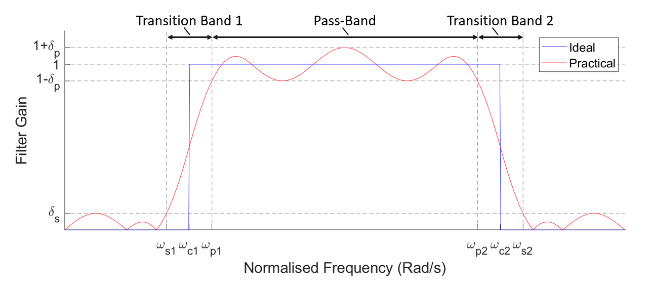
An image to reemphasize how the properties defined in the table above relate to a plot of a pass-band filters frequency response. — An example of the general parameters required to define a pass-band filter.

This defines how much the filter amplitude is allowed to deviate in the pass- and stop- regions, as well as an allowed blurring of the boundary between these regions. This blurring of boundaries causes the vertical cut-off points to become more gradual slopes, resulting in new regions known as the transition bands.

It may be noticed that the ideal cut-off frequencies, $\omega_{c1}$ and $\omega_{c2}$, are located towards the centre of the transition band, meaning that as the transition band widens it eats into both the pass- and stop-bands. It is also important to note that in the transition band regions, signals are neither fully passed nor fully removed by the filter, meaning that some distortion may occur for frequencies found within these regions. For this reason, it is typical to ensure that the desired frequencies are kept firmly within the pass-band region.

In this exercise the unknown signal has some key properties that will help guide the selection of these parameters. You may assume that the ideal pass-band (located between $\omega_{c1}$ and $\omega_{c2}$) is 10Hz wide and centred on the carrier frequency of the AM signal. The transition bands should be specified to be 6Hz wide.

These specifications have been selected to provide a tight fit over all students' AM signals, ensuring that everyone achieves a clean result regardless of any nearby interference frequencies. In reality, the filter could likely be defined more loosely for your signal; however, these guidelines have been chosen to aid the marking process and ensure that each individual's exercise maintains the same level of difficulty.

Using these criteria, and based on the message frequencies already identified…

Find the normalized lower cut-off frequency, $f_{c1}$.
Find the normalized lower stop-band edge frequency, $f_{s1}$.
Find the normalized lower pass-band edge frequency, $f_{p1}$.
Find the normalized upper cut-off frequency, $f_{c2}$.
Find the normalized upper stop-band edge frequency, $f_{s2}$.
Find the normalized upper pass-band edge frequency, $f_{p2}$.

You can enter these frequencies into the FIR Skill Tool to verify your answers.

The Windowing Method

Once a filters approximation limits have been specified, the coefficients must be identified to actually implement the filter. There are many ways to approach this step, however, in this lab we will utilize a method known as the windowing method.

Windowing the Coefficients

The ideal filter coefficients defined in Equation \eqref{eq:DiscreteIdealTime} were infinite in length and non-causal. We can solve these issues by windowing and time-shifting the ideal-case coefficients.

This is effectively like taking a reduced snapshot of the coefficient values within some pre-defined range. By doing this, we limit the number coefficients down to a finite number of entries. A time-shift is then also required to ensure that the windowed FIR filter is causal (meaning that an output will not be produced before any input arrives).

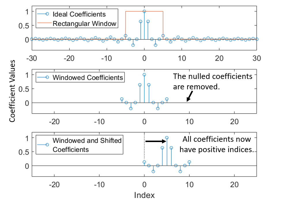
Three subplots, with the first showing in infinite length non-causal set of filter coefficients and a rectangular window. The second shows the result of applying (multiplying) this window with the original signal. The final plot shows how this newly truncated signal can be shifted by half the window width to result in coefficients that only occur index values greater than 0. — Plots showing how an infinite length, non-causal set of filter coefficients (top) may be truncated (middle) and shifted (bottom) to result in a finite length causal set of filter coefficients.

From it can be noted that the dominant coefficients (with most influence on the signal) have been preserved, however approximation error will have been introduced by failing to include the coefficients outside of the window. As the window is made wider (to include more of the coefficients), the total influence of any missing coefficients is further reduced, improving the approximation accuracy of the resulting filter.

Mathematically, this process may be defined using Equation \eqref{eq:WindowBasic}, where $h[n]$ represents the windowed filter coefficients, $W[n]$ represents the window itself (a rectangular pulse in the case of ), and $h_i[n]$ represents the original infinite-length non-causal filter coefficients.

\[\begin{equation} h[n]=W[n]h_i[n] \label{eq:WindowBasic} \end{equation}\]

By windowing and shifting the coefficients, we now have a set of finite coefficients that define a causal linear filter. This new windowed filter only approximates our original ideal filter. The quality of this approximation will depend largely upon the properties of the chosen window function itself.

Selecting Window Functions

So far, we have assumed that the window function, $W[n]$, is a basic rectangular (or boxcar) function. This works alright in some cases, however it often produces a poor performance in practical filters, due to the hard edge at the boundaries of the window.

By appropriately shaping the window function, it is possible to reduce the ripple (and thus approximation error) and control the size of the filters transition band. There are many functions that could be used to window a signal, and selecting the appropriate one will require the balancing of different tradeoff such as filter length, band ripple and transition band width.

Some of the more common windowing functions are as follows:

Name	Window Function	Approximate Main Lobe Width	Peak Approximation Error, $20\log(\delta)$ (dB)
Rectangular	$W[n]=\left\{\begin{array}{ll}1, & \mbox{if $0 < n < M$}.\\0, & \mbox{otherwise}.\end{array}\right.$	$\frac{4\pi}{M+1}$	-21
Hann	$W[n]=\left\{\begin{array}{ll}0.5-0.5\cos{(\frac{2n\pi}{M})}, & \mbox{if $0\leq n\leq M$}.\\0, & \mbox{otherwise}.\end{array}\right.$	$\frac{8\pi}{M}$	-44
Hamming	$W[n]=\left\{\begin{array}{ll}0.54-0.46\cos{(\frac{2n\pi}{M})}, & \mbox{if $0\leq n\leq M$}.\\0, & \mbox{otherwise}.\end{array}\right.$	$\frac{8\pi}{M}$	-53

The approximate main lobe width of a windowing function (measured in radians per second) is closely related to the width of the transition band. Therefore, for any given transition-band width, the total number of coefficients required, denoted as $M$, can be determined by setting the approximate main lobe width equal to the desired transition-band width.

The peak approximation error of the windowing function determines the amount of ripple observed in both the pass-band and stop-band. Since the ideal filter is expected to have infinite attenuation in the stop-band (i.e., the signal should be completely blocked), any real filter designed with a windowing function cannot achieve this ideal as the windowing function’s peak approximation error sets a limit on the attenuation in the stop-band. As a result, the actual stop-band attenuation of the filter will be equal to the peak approximation error of the windowing function.

Assume that the maximum amplitude of any signal present within the stop-band region of the filter ($\delta_s$) should be less than 0.005, and that the maximum pass-band ripple doesn’t matter (meaning it makes sense to also set it to $\delta_p=0.005$ to relax the limits as much as possible), …

Calculate the maximum peak approximation error in dB required to ensure that the stop-band maximum amplitude requirement is met.
From your result in the previous question, use the table of windowing functions above to select the most suitable windowing function.
Calculate the required window width, $M$, using the filter properties defined in Exercise 4.

You may, again, enter these values into the FIR Skill Tool to check your answers.

Creating the filter

By this stage, all the elements required to create a practical filter have been defined.

The process to produce the filter coefficients is therefore as follows:

Derive the expression for the ideal filter coefficients with respect to $n$, the coefficient index.
Time-shift the expression by half the window width ($M$) to ensure that the final set of windowed coefficients will be causal.
Produce a trimmed set of time-shifted coefficients down to the range $0<n<=M$ - i.e. only apply the expression from step 2 for this limited set of $n$.
Calculate the window values for each $n$ index.
Multiply the coefficient values with the window values.

Steps 4 and 5 can be omitted if using a rectangular window.

Once the coefficients of the filter have been defined, a signal may be filtered by simply convolving the coefficients ($h$) with the signal ($x$) using conv(h,x). As convolution will extend the length of the signal by the filters length, you will need to generate a new time sequence of correct length to be able to plot the filtered signal against time.

Filter Coefficients Function Challenge

Breaking this approach into pieces, we will first create a function to implement steps 1 to 3.

Modify your ideal filter coefficients equation that was derived in the ‘Ideal Band-Pass Filters’ exercise to time-shift the expression by $M/2$ samples, where $M$ is a variable in the equation.
Write a function to implement this equation, called calcIdealCoefficients(), which takes $W_{c1}$, $W_{c2}$ and $M$ and returns a time-shifted length-trimmed vector of coefficients, $h[n]$.

Tips

Time-Shifting the Ideal Filter Coefficients:

Recall that time-shifting a discrete signal by $M/2$ samples can be achieved by modifying the index of the impulse response.
For example, if the original ideal filter coefficients were defined as $h[n] = \text{sin}(n)$, the time-shifted version can be written as:
$h[n] = \text{sin}\left(n - M/2\right)$

Angular Frequency vs Frequency

Your frequencies you have measured are not in angular frequency, but this function requires angular frequencies.
Don’t forget to convert between angular frequency and normal frequency before passing values into the function.

Function Implementation:

You can test the calcIdealCoefficients() by using it to generate filter coefficients with known properties and then plotting these coefficients with your FFT function (or the more complex built in freqz(h) function which will help normalize the filter gain axis but also normalizes the frequency axis).

Now we have a way to calculate the trimmed and time-shifted coefficients, we need to find the window coefficients.

As before, write a function to implement the selected windowing function called calcWindow() that takes $M$ as an argument and returns the vector $W[n]$.

Use calcIdealCoefficients() and calcWindow() to generate two vectors, h_trimmed and W, multiplying them together to yield your filter coefficients h.

Now you have your filter, it is time to apply it to the signal to see if you can retrieve the original AM signal. If successful, then well done - this is not an easy task.

Claiming the Skill

Now that you have the filter properties, window properties and filter coefficients, you can use the FIR Skill Tool to generate a set of skill sheets that may be uploaded to Moodle. Make sure that the username is still entered correctly at the top of the form - again, if working in pairs both of you should be using only one of your usernames at this stage.

The filter coefficients dropdown allows you to select any variable in your workspace, so make sure that you have the coefficients generated, and then use the dropdown to select them.

Clicking check results will highlight any entries that have issues or need to be re-calculated.

Once everything is correct, click ‘Generate Skill Sheet’ and it will place two PNG images in your folder, one called page_1.png and the other called page_2.png. If all answers were correct then you should see an FIR skills badge in the top corner of the pages. Note, if nothing happens, check the MATLAB command window for any messages.

To use these skill sheets, simply log into Mahara and upload both pages into the Mahara page where you wish to claim the skill. If working in pairs, both members must also add text to state who their partner was (name and username).

Finally, the FIR Skill Tool includes a ‘custom’ mode (see the exercise dropdown), allowing you to create skill sheets for other filter designs that you have worked on. These will not be automatically verified before page generation.

Property	Symbol	Definition
Sampling Frequency	\(f_s\)	The rate at which the data is sampled. While this value will not directly impact the filter coefficients, it will determine what real frequencies are represented by the normalized frequencies used during the design process.
Pass-Band Edge Frequency	\(f_p\)	The frequency where the boundary between the transition band region and the pass-band region is located.
Stop-Band Edge Frequency	\(f_s\)	The frequency where the boundary between the transition band region and the stop-band region is located.
Pass-Band Ripple	\(f_p\)	The maximum amount of fluctuation from the nominal value that is allowed within the pass-band region.
Stop-Band Ripple	\(f_s\)	The maximum amount of fluctuation from the nominal value that is allowed within the stop-band region.

Name	Window Function	Approximate Main Lobe Width	Peak Approximation Error, $20\log(\delta)$ (dB)
Rectangular	\(W[n]=\left\{\begin{array}{ll}1, & \mbox{if $0 < n < M$}.\\0, & \mbox{otherwise}.\end{array}\right.\)	\(\frac{4\pi}{M+1}\)	-21
Hann	\(W[n]=\left\{\begin{array}{ll}0.5-0.5\cos{(\frac{2n\pi}{M})}, & \mbox{if $0\leq n\leq M$}.\\0, & \mbox{otherwise}.\end{array}\right.\)	\(\frac{8\pi}{M}\)	-44
Hamming	\(W[n]=\left\{\begin{array}{ll}0.54-0.46\cos{(\frac{2n\pi}{M})}, & \mbox{if $0\leq n\leq M$}.\\0, & \mbox{otherwise}.\end{array}\right.\)	\(\frac{8\pi}{M}\)	-53