
PGF/TikZ is a pair of languages for producing vector graphics (e.g., technical illustrations and drawings) from a geometric/algebraic description, with standard features including the drawing of points, lines, arrows, paths, circles, ellipses and polygons. PGF is a lower-level language, while TikZ is a set of higher-level macros that use PGF. The top-level PGF and TikZ commands are invoked as TeX macros, but in contrast with PSTricks, the PGF/TikZ graphics themselves are described in a language that resembles MetaPost. Till Tantau is the designer of the PGF and TikZ languages, who is also the main developer of the only known interpreter for PGF and TikZ, which is written in TeX. PGF is an acronym for “Portable Graphics Format”. TikZ was introduced in version 0.95 of PGF, and it is a recursive acronym for “TikZ ist kein Zeichenprogramm” (German for “TikZ is not a drawing program”).
This section I will introduce how to write in LaTeX to make TikZ graphs. I will include 4 examples with code to show you the most important features of TikZ and you should be able to produce many graphs after the four examples.
You can use TikZ in LaTeX, the package is tikz. To include the package:
\usepackage{tikz}If you want to draw a tikz graph in LaTeX, use:
\begin{tikzpicture}
    code here
\end{tikzpicture}
The fowllowing examples demonstrates: * how to draw simple shapes, arrows, arrange text on graphs; * how to draw simple 3D shapes and a reference to make complicated graphs; * how to make a flow chart; * how to make a graph by loading data from a .csv file.
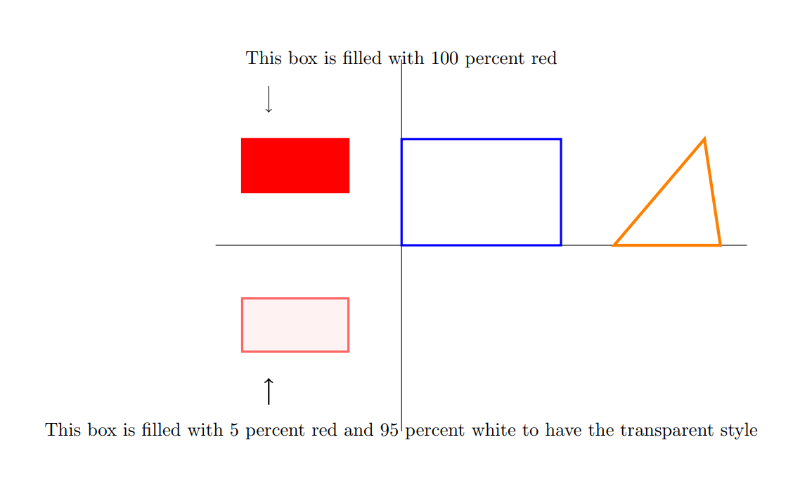
This graph shows how to draw simple shapes and arrows and text using tikz.
The source code:
\documentclass{article}
\usepackage{tikz}
\begin{document}
\begin{tikzpicture}
 %set the coordinates
  \draw (-3.5,0) -- (6.5,0);
  \draw (0,-3.5) -- (0,3.5);

% draw a rectangle
\draw[blue, very thick] (0,0) rectangle (3,2);
% draw a rectangle with colour fill and colour edge
\filldraw[color=red, fill=red, very thick](-1,1) rectangle(-3,2);
% draw a rectangle with colour fill 5% red edges: 60% red colour
\filldraw[color=red!60, fill=red!5, very thick](-1,-1) rectangle(-3,-2);
% draw a triangle: connect all the three points:
\draw[orange, ultra thick] (4,0) -- (6,0) -- (5.7,2) -- cycle;

% put some arrows on the graph:
% the arrow pointing towards the red rectangle
\draw[->] (-2.5,3) -- (-2.5,2.5);
% the arrow pointing towards the pink fill rectangle
\draw[->,thick] (-2.5,-3) -- (-2.5,-2.5);

% add some text
\node at (0,-3.5) {This box is filled with 5 percent red and 95 percent white to have the transparent style };

\node at (0,3.5) {This box is filled with 100 percent red};
\end{tikzpicture}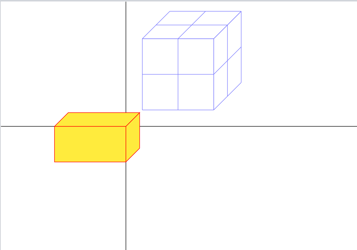
\end{document}This example shows how to draw 3D cuboids and grids.
Code :
\documentclass{standalone}
\usepackage{tikz}
\begin{document}
\begin{tikzpicture}

% this draw the help lines (light lines at the background)
% \draw[help lines] (-6,-2) grid (6,4);
 %set the coordinates
  \draw (-3.5,0) -- (6.5,0);
  \draw (0,-3.5) -- (0,3.5);

% method 1: the yellow cuboid:
\pgfmathsetmacro{\cubex}{2}
\pgfmathsetmacro{\cubey}{1}
\pgfmathsetmacro{\cubez}{1}
\draw[red,fill=yellow] (0,0,0) -- ++(-\cubex,0,0) -- ++(0,-\cubey,0) -- ++(\cubex,0,0) -- cycle;
\draw[red,fill=yellow] (0,0,0) -- ++(0,0,-\cubez) -- ++(0,-\cubey,0) -- ++(0,0,\cubez) -- cycle;
\draw[red,fill=yellow] (0,0,0) -- ++(-\cubex,0,0) -- ++(0,0,-\cubez) -- ++(\cubex,0,0) -- cycle;


% method 2: the cube
\foreach \x in{2,...,4}
{   \draw[blue!50] (2,\x ,4) -- (4,\x ,4);
    \draw[blue!50] (\x ,2,4) -- (\x ,4,4);
    \draw[blue!50] (4,\x ,4) -- (4,\x ,2);
    \draw[blue!50] (\x ,4,4) -- (\x ,4,2);
    \draw[blue!50] (4,2,\x ) -- (4,4,\x );
    \draw[blue!50] (2,4,\x ) -- (4,4,\x );
}

\end{tikzpicture}
\end{document}
An interesting reading about some fancy 3D shapes: https://tex.stackexchange.com/questions/29877/need-help-creating-a-3d-cube-from-a-2d-set-of-nodes-in-tikz
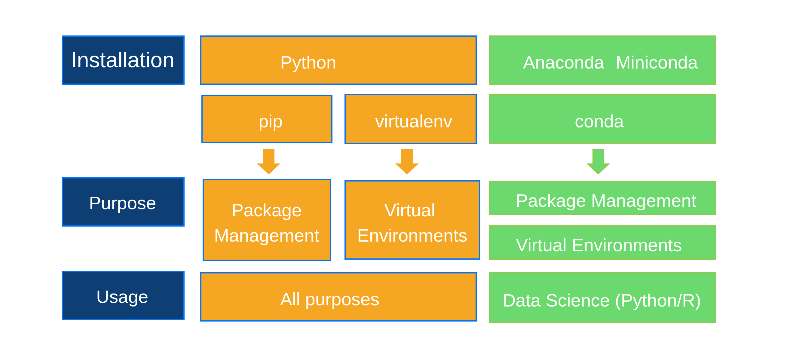
A flow chart I created for anaconda training. This graph is created by using TikZ.
\tikzset{every picture/.style={line width=0.75pt}} %set default line width to 0.75pt

\begin{tikzpicture}[x=0.75pt,y=0.75pt,yscale=-1,xscale=1]
%uncomment if require: \path (0,300); %set diagram left start at 0, and has height of 300

%Shape: Rectangle [id:dp6456533430603446]
\draw  [color={rgb, 255:red, 4; green, 115; blue, 247 }  ,draw opacity=1 ][fill={rgb, 255:red, 13; green, 63; blue, 116 }  ,fill opacity=1 ] (52,30) -- (153,30) -- (153,70) -- (52,70) -- cycle ;
%Shape: Rectangle [id:dp5542532442985997]
\draw  [color={rgb, 255:red, 4; green, 115; blue, 247 }  ,draw opacity=1 ][fill={rgb, 255:red, 13; green, 63; blue, 116 }  ,fill opacity=1 ] (52,148) -- (153,148) -- (153,188) -- (52,188) -- cycle ;
%Shape: Rectangle [id:dp48148077053260474]
\draw  [color={rgb, 255:red, 4; green, 115; blue, 247 }  ,draw opacity=1 ][fill={rgb, 255:red, 13; green, 63; blue, 116 }  ,fill opacity=1 ] (52,226) -- (153,226) -- (153,266) -- (52,266) -- cycle ;
%Shape: Rectangle [id:dp9870710123964177]
\draw  [color={rgb, 255:red, 4; green, 115; blue, 247 }  ,draw opacity=1 ][fill={rgb, 255:red, 245; green, 166; blue, 35 }  ,fill opacity=1 ] (167,30) -- (396,30) -- (396,70) -- (167,70) -- cycle ;
%Shape: Rectangle [id:dp9025864616283901]
\draw  [color={rgb, 255:red, 140; green, 201; blue, 76 }  ,draw opacity=1 ][fill={rgb, 255:red, 107; green, 217; blue, 110 }  ,fill opacity=1 ] (407,30) -- (595,30) -- (595,70) -- (407,70) -- cycle ;
%Shape: Rectangle [id:dp04614999842800893]
\draw  [color={rgb, 255:red, 4; green, 115; blue, 247 }  ,draw opacity=1 ][fill={rgb, 255:red, 245; green, 166; blue, 35 }  ,fill opacity=1 ] (168,79.5) -- (276,79.5) -- (276,118.5) -- (168,118.5) -- cycle ;
%Shape: Rectangle [id:dp6636931384454097]
\draw  [color={rgb, 255:red, 4; green, 115; blue, 247 }  ,draw opacity=1 ][fill={rgb, 255:red, 245; green, 166; blue, 35 }  ,fill opacity=1 ] (287,78.5) -- (396,78.5) -- (396,119.5) -- (287,119.5) -- cycle ;
%Shape: Rectangle [id:dp6230448237562309]
\draw  [color={rgb, 255:red, 140; green, 201; blue, 76 }  ,draw opacity=1 ][fill={rgb, 255:red, 107; green, 217; blue, 110 }  ,fill opacity=1 ] (407,79) -- (595,79) -- (595,119) -- (407,119) -- cycle ;
%Shape: Rectangle [id:dp6699050665048052]
\draw  [color={rgb, 255:red, 4; green, 115; blue, 247 }  ,draw opacity=1 ][fill={rgb, 255:red, 245; green, 166; blue, 35 }  ,fill opacity=1 ] (169,149.5) -- (275,149.5) -- (275,216.5) -- (169,216.5) -- cycle ;
%Shape: Rectangle [id:dp14651239788062198]
\draw  [color={rgb, 255:red, 4; green, 115; blue, 247 }  ,draw opacity=1 ][fill={rgb, 255:red, 245; green, 166; blue, 35 }  ,fill opacity=1 ] (287,150.5) -- (399,150.5) -- (399,215.5) -- (287,215.5) -- cycle ;
%Shape: Rectangle [id:dp8617603066811956]
\draw  [color={rgb, 255:red, 4; green, 115; blue, 247 }  ,draw opacity=1 ][fill={rgb, 255:red, 245; green, 166; blue, 35 }  ,fill opacity=1 ] (167,227) -- (396,227) -- (396,267) -- (167,267) -- cycle ;
%Shape: Rectangle [id:dp5911896335069105]
\draw  [color={rgb, 255:red, 140; green, 201; blue, 76 }  ,draw opacity=1 ][fill={rgb, 255:red, 107; green, 217; blue, 110 }  ,fill opacity=1 ] (407,151) -- (595,151) -- (595,178.5) -- (407,178.5) -- cycle ;
%Shape: Rectangle [id:dp7844988104186317]
\draw  [color={rgb, 255:red, 140; green, 201; blue, 76 }  ,draw opacity=1 ][fill={rgb, 255:red, 107; green, 217; blue, 110 }  ,fill opacity=1 ] (407,188) -- (595,188) -- (595,215.5) -- (407,215.5) -- cycle ;
%Shape: Rectangle [id:dp38292829163657305]
\draw  [color={rgb, 255:red, 140; green, 201; blue, 76 }  ,draw opacity=1 ][fill={rgb, 255:red, 107; green, 217; blue, 110 }  ,fill opacity=1 ] (407,227) -- (595,227) -- (595,268.5) -- (407,268.5) -- cycle ;
%Down Arrow [id:dp7227684014917184]
\draw  [color={rgb, 255:red, 245; green, 166; blue, 35 }  ,draw opacity=1 ][fill={rgb, 255:red, 245; green, 166; blue, 35 }  ,fill opacity=1 ] (215,136.5) -- (219.25,136.5) -- (219.25,124.5) -- (227.75,124.5) -- (227.75,136.5) -- (232,136.5) -- (223.5,144.5) -- cycle ;
%Down Arrow [id:dp26834762190164674]
\draw  [color={rgb, 255:red, 245; green, 166; blue, 35 }  ,draw opacity=1 ][fill={rgb, 255:red, 245; green, 166; blue, 35 }  ,fill opacity=1 ] (330,136.5) -- (334.25,136.5) -- (334.25,124.5) -- (342.75,124.5) -- (342.75,136.5) -- (347,136.5) -- (338.5,144.5) -- cycle ;
%Down Arrow [id:dp007482605047406388]
\draw  [color={rgb, 255:red, 140; green, 201; blue, 76 }  ,draw opacity=1 ][fill={rgb, 255:red, 107; green, 217; blue, 110 }  ,fill opacity=1 ] (489,136.5) -- (493.25,136.5) -- (493.25,124.5) -- (501.75,124.5) -- (501.75,136.5) -- (506,136.5) -- (497.5,144.5) -- cycle ;

% Text Node
\draw (58,40) node [anchor=north west][inner sep=0.75pt]  [color={rgb, 255:red, 255; green, 255; blue, 255 }  ,opacity=1 ] [align=left] {\begin{undefined}
{\large Installation}
\end{undefined}
};
% Text Node
\draw (73,160) node [anchor=north west][inner sep=0.75pt]  [color={rgb, 255:red, 255; green, 255; blue, 255 }  ,opacity=1 ] [align=left] {\begin{undefined}
Purpose
\end{undefined}
};
% Text Node
\draw (79,238) node [anchor=north west][inner sep=0.75pt]  [color={rgb, 255:red, 255; green, 255; blue, 255 }  ,opacity=1 ] [align=left] {\begin{undefined}
Usage
\end{undefined}
};
% Text Node
\draw (232,43) node [anchor=north west][inner sep=0.75pt]  [color={rgb, 255:red, 255; green, 255; blue, 255 }  ,opacity=1 ] [align=left] {\begin{undefined}
Python
\end{undefined}
};
% Text Node
\draw (434,43) node [anchor=north west][inner sep=0.75pt]  [color={rgb, 255:red, 255; green, 255; blue, 255 }  ,opacity=1 ] [align=left] {\begin{undefined}
Anaconda
\end{undefined}
};
% Text Node
\draw (511,43) node [anchor=north west][inner sep=0.75pt]  [color={rgb, 255:red, 255; green, 255; blue, 255 }  ,opacity=1 ] [align=left] {\begin{undefined}
Miniconda
\end{undefined}
};
% Text Node
\draw (214,92) node [anchor=north west][inner sep=0.75pt]  [color={rgb, 255:red, 255; green, 255; blue, 255 }  ,opacity=1 ] [align=left] {\begin{undefined}
pip
\end{undefined}
};
% Text Node
\draw (311,92) node [anchor=north west][inner sep=0.75pt]  [color={rgb, 255:red, 255; green, 255; blue, 255 }  ,opacity=1 ] [align=left] {\begin{undefined}
virtualenv
\end{undefined}
};
% Text Node
\draw (477,92) node [anchor=north west][inner sep=0.75pt]  [color={rgb, 255:red, 255; green, 255; blue, 255 }  ,opacity=1 ] [align=left] {\begin{undefined}
conda
\end{undefined}
};
% Text Node
\draw (177,166) node [anchor=north west][inner sep=0.75pt]  [color={rgb, 255:red, 255; green, 255; blue, 255 }  ,opacity=1 ] [align=left] {\begin{minipage}[lt]{62.25pt}\setlength\topsep{0pt}
\begin{center}
Package
\end{center}
\begin{undefined}
Management
\end{undefined}

\end{minipage}};
% Text Node
\draw (296,166) node [anchor=north west][inner sep=0.75pt]  [color={rgb, 255:red, 255; green, 255; blue, 255 }  ,opacity=1 ] [align=left] {\begin{minipage}[lt]{65.07pt}\setlength\topsep{0pt}
\begin{center}
Virtual \\Environments
\end{center}

\end{minipage}};
% Text Node
\draw (232,240) node [anchor=north west][inner sep=0.75pt]  [color={rgb, 255:red, 255; green, 255; blue, 255 }  ,opacity=1 ] [align=left] {\begin{undefined}
All purposes
\end{undefined}
};
% Text Node
\draw (428,158.04) node [anchor=north west][inner sep=0.75pt]  [color={rgb, 255:red, 255; green, 255; blue, 255 }  ,opacity=1 ] [align=left] {\begin{undefined}
Package Management
\end{undefined}
};
% Text Node
\draw (428,195.04) node [anchor=north west][inner sep=0.75pt]  [color={rgb, 255:red, 255; green, 255; blue, 255 }  ,opacity=1 ] [align=left] {\begin{undefined}
Virtual Environments
\end{undefined}
};
% Text Node
\draw (417,241.04) node [anchor=north west][inner sep=0.75pt]  [color={rgb, 255:red, 255; green, 255; blue, 255 }  ,opacity=1 ] [align=left] {\begin{undefined}
Data Science (Python/R)
\end{undefined}
};


\end{tikzpicture}
There are many resources about how to draw flow charts using tikz. Try to google it and find one example to try it yourself.
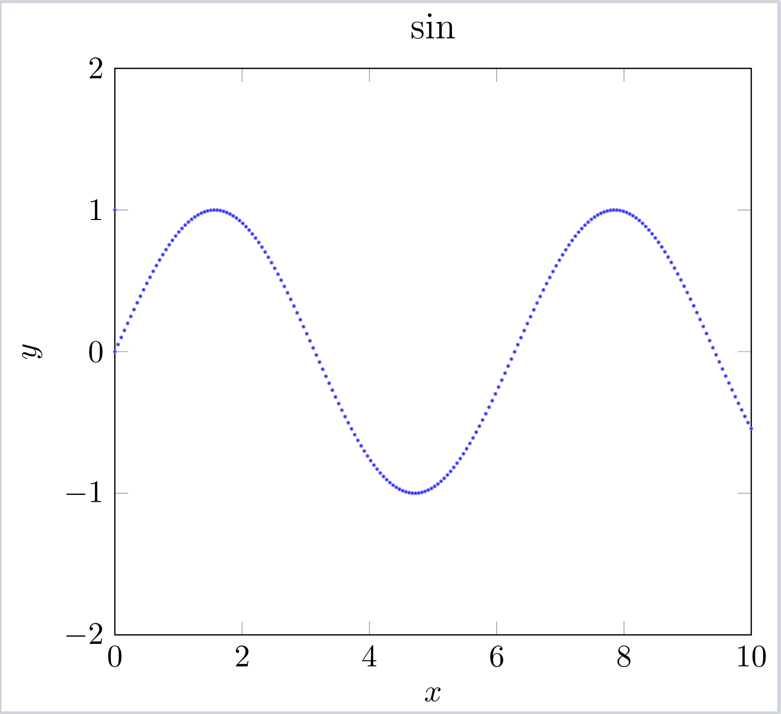
This is a simple graph of the \(\sin\) function. The purpose of this example is to show how you read in data from a .csv file to produce graphs using TikZ. This could be really useful for us when we want to produce high quality graphs for journals.
Code :
\documentclass{standalone}

% User packages:
% ======================================================================
\usepackage{amsmath}
\usepackage{amsfonts}
\usepackage{amssymb}
\usepackage{graphicx}
\usepackage{epsfig}
\usepackage[hang,nooneline]{subfigure}
\usepackage[normalem]{ulem}
\usepackage{color}
\usepackage{braket}
\usepackage{hyperref}
\usepackage{todonotes}
\usepackage{algorithm}
\usepackage{multirow}
\usepackage{hhline}
\usepackage{shortvrb}
\usepackage{cprotect}
\usepackage[noend]{algpseudocode}
\usepackage{overpic}
\usepackage{cleveref}

% Tikz plot
\usepackage{csvsimple}
\usepackage{tikz}
\usepackage{pgfplots}
\usepgfplotslibrary{colorbrewer}
\definecolor{seabornblue}{rgb}{0.2980392156862745, 0.4470588235294118, 0.6901960784313725}

\makeatletter

\usetikzlibrary{external}
% Comment out the next three lines for faster compilation time
\usepgfplotslibrary{external}
\pgfplotsset{compat=newest}
\tikzexternalize[optimize=false] % or false

\tikzset{external/system call= {lualatex
                           -enable-write18
                           -halt-on-error
                           -shell-escape
                           -synctex=1
                           -interaction=nonstopmode
                           -jobname "\image" "\texsource"}}

\begin{document}

\tikzsetnextfilename{1}

\begin{tikzpicture}

\begin{axis}[scale only axis=true, width=0.33*8.5in, height=2.5in, xmin=0, xmax=10, ymin=-2, ymax=2, enlargelimits=false, xlabel={$x$}, ylabel={$y$}, title={\large $\sin$}]
\node  at (-0.15*10^5,1.05*250) {\Large (a)};
% plot the loaded data from data.csv
\addplot+[blue!60, only marks, mark size=0.4] table [col sep=comma] {data.csv};
\end{axis}

\end{tikzpicture}
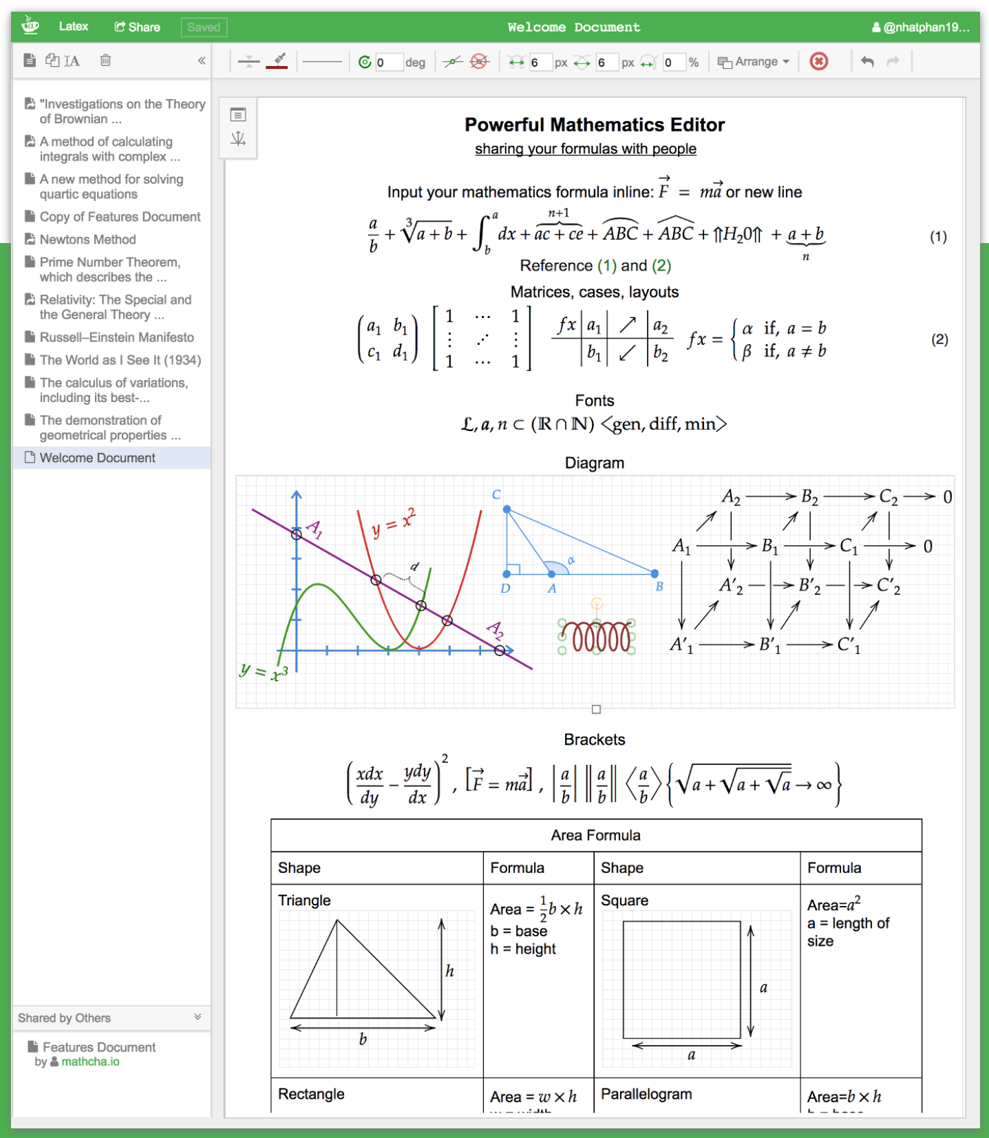
\end{document}TikZ is powerful but it can be a little bit complicated. Especially for simple graphs. (Even though I personally love writing codes for simple graphs.) It is much easier to draw simple graphs using some online tikz editors. (Many also include a desktop notebook). In this tutorial, I introduce one powerful but easy to use online editors: Matcha
Quick access editor without the requirement of knowing latex nor tikz. Maths formula and graphs can be exported as Image (PNG), Vector (SVG), or printed out as PDF. It also supports the export or Import LATEX for Math Mode.
Try TikZ on Overleaf or locally on TeXMaker. Or use Matcha.io to create some simple shapes or design a simple flow chart.
Here are a few figures I found online, can you try to reproduce some of them?
Figure 1: 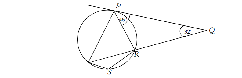
Figure 2: 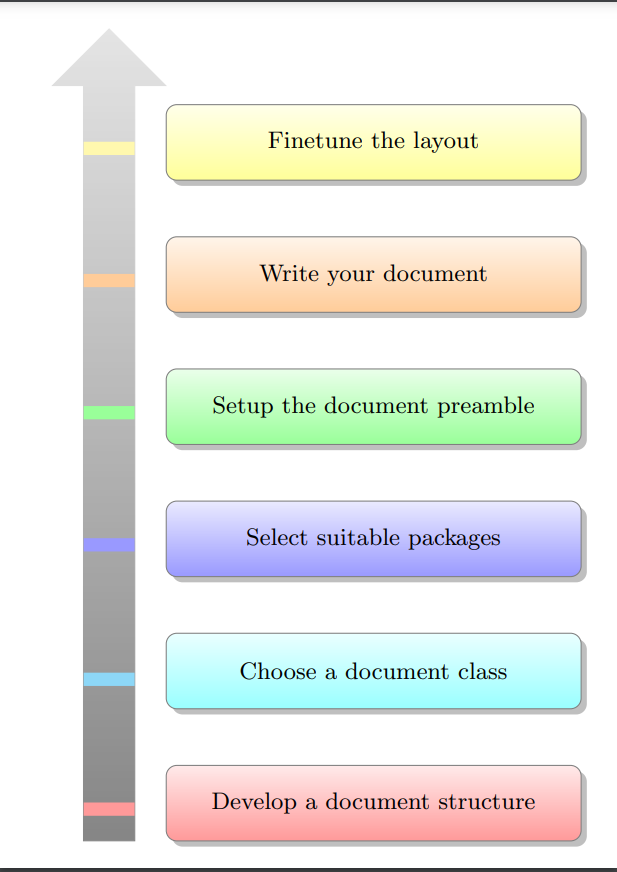
Hit: Can you do the simple flowchart first? Then try to add some colour. Solution to Figure 2: https://texample.net/tikz/examples/smart-priority/
Figure 3 (If you are crazy try this) 
Solution to Figure 3: https://texample.net/tikz/examples/totoro/
The TikZ manual: https://tikz.dev/
The mathcha website: https://www.mathcha.io/
TikZ graphics tutorials:
TikZ package introduction: https://www.overleaf.com/learn/latex/TikZ_package
Online platform: https://www.mathcha.io/ Use the online editor: https://www.mathcha.io/
Desktop Mathcha Notebook: https://www.mathcha.io/notebook/ Ubuntu (16+): https://snapcraft.io/install/math-notebook/ubuntu $ sudo snap install math-notebook