home
| CV |
| Research |
| Teaching |
| Contact |
| NASA ADS link |
| Google Scholar link |
| Photography |
| Amusements |
| Useful Links |
| The RemarXiv Research Blog |
| Iron Line Variability of Discoseismic C-Modes |
This work was done with my 2012 SURF student Iryna Butsky, and has been accepted for publication in MNRAS, and is available on the arXiv. The summary below was prepared by Iryna. A link to the relavent raytracing code is also below. X-ray emissions from accretion disks around black holes are modulated by quasi periodic oscillations (QPOs). The cause of these oscillations is not yet understood. We propose that low frequency QPOs may be caused by corrugation modes, which are vertical discoseismic oscillations in the inner region of the accretion disk. Fe Kα emission profiles are a powerful tool for probing the inner structure of the disk. X-ray fluorescence creates a particularly sharp emission profile, while Doppler boosting and gravitational redshift cause a spread and a bimodal nature of this emission profile. With this project, we attempt to establish a dependency of the Kα emission spectrum on the phase of the QPO.
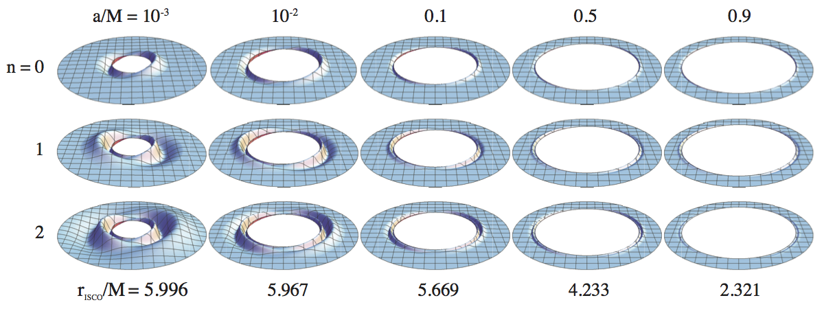
Corrugation modes are natural oscillation modes of accretion disks trapped between rISCO and the inner vertical resonance (rIVR), which strongly modify the inner structure of the disk. The corrugation modes with radial nodes n = 0, 1, 2 for black holes with spin a/M = 0.001, 0.01, 0.1, 0.5, 0.9 . With higher spin, the propagation region of the modes are greatly reduced. Raytracing As a photon escapes the gas of an accretion disk, its path is influenced by gravitational bending of light rays, gravitational redshift, and the relativistic Dopler effect before it reaches the observer. Since this is a time reversible process, we employ a technique called raytracing, which follows the trajectory of a photon from the observer to the accretion disk. We assume the accretion disk to be in a Keplerian orbit around the black hole. Therefore, the gas moving away from the observer will be redshifted, and likewise the gas moving towards the observer will appear blueshifted.
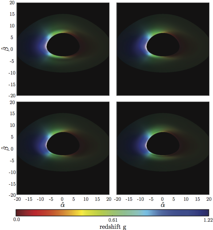
Above is an example disk images as a function of the phase of the perturbation. Moving clockwise from the top left corner, the oscillation phase increases by π/2. The color represents the redshift, while the brightness represents the intensity. This is a representation of an accretion disk for a black hole with spin a/M = 0.001, μo = 0.5, and an arbitrarily chosen r=20M. These images were created assuming a limb brightening law, f(μem) = log(1 + 1/μem), for the angular emissivity. Raytracing To perform the ratytracing, we implement a new semi-analytic ray-tracing method to model and visualize accretion disks perturbed with corrugation modes. Our code enables us to generate the observed line profile of the Fe Kα emission lines as a function of the corrugation mode phase. This information is useful in predicting the signature for observations obtained from X-Ray telescopes and in verifying the strength of the Fe Kα QPO connection. We consider four parameters as arguments: a, the unitless black hole spin, μo, the cosine of the angle of inclination to the observer, the maximum distance (in units of black hole mass) from the black hole that we want to consider in our calculations, and the resolution of the grid to be returned. This information is used to generate a matrix which represent pixels seen by the observer. Each pixel contains contains information about the position vector (in polar coordinates), the momentum vector, the combined redshift value (g), and whether or not the photon hit the accretion disk. From this information, we can generate images of an accretion disk, as seen above. You can download a version of the code here. With our code, we are able to predict an X-ray emission signature of an accretion disk perturbed with corrugation modes. Observations with sufficient spectral and temporal resolution will be able to determine whether or not LFQPOs are in fact caused by c-modes. If corrugation modes are present within the inner accretion disk, we will be able to probe them by phase stacking the received signal. The spectral ranges and frequencies over which this variability is seen for corrugation modes can act as a probe of black hole spin parameter complementary to existing spin constraints from thermal and broadened iron-line observations
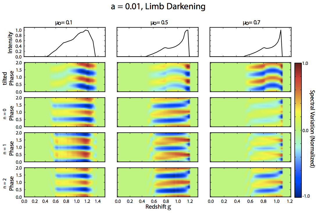
The first row represents the unperturbed intensity as a function of the redshift. The remaining panels represent the deviation from the average intensity as a function of phase.The second row represents the signature of a tilted disk that is unperturbed but precessing at a frequency at the QPO frequency. The bottom three panels show the signature of c-mode perturbations with nodes n = 0, 1, 2.
Instructions for using qpotrace For faster computational time the raytracing segment of our program is written in C. However, to improve user interface, the C code is “wrapped” and accessible through Python. To generate an accretion disk, you only need to modify the gen_rtr.py file. The parameters you will need to adjust are: ·a – the black hole spin in units of BH mass. Valid values are in the range 0 < a < 1 ·mu_o – the cosine of the inclination angle (to the observer). Accepts values of 0 <= mu_o <= 1 ·res – the resolution, where res x res determines the number of pixels to be returned. We suggest starting with values of res ~ 100 for trial runs and testing. Note that with increasing spin, a higher resolution is required to properly resolve any perturbations. · rout – the arbitrary edge of the accretion disk, in units of BH mass. This value decreases with increasing black hole spin parameter. After the raytracing is finished running, it will use Python’s cPickle module to create an output file called (NAME). The outputs are: a, res, mu_o, etc. etc. in that order. To retrieve data from the file, first import cPickle and open the desired file in python: import cPickle as pickle myfile = open(‘NAME’, ‘r’) Then, to access the individual data elements, call res = pickle.load(myfile) ipmax = pickle.load(myfile) a = pickle.load(infile) mu_o = pickle.load(infile) x = pickle.load(infile) # The position vector (t,r,phi,theta) kvec = pickle.load(infile) # The velocity vector hit = pickle.load(infile) # 1 = in the accretion disc, # 0=outside the disc g = pickle.load(infile) # The redshift of a given particle emcos = pickle.load(infile) # The cosine of the emission angle close(myfile)
|