This Document contains keywords, examples and contact information. The code is organised in a series of modules, each module has a different activity.

Modules in the Metadise Code

Meta, Property, Stackgen, Miller, Step, Minimise, Flexible, Scan, IR, MD, MC, Phon Match Chaos Segregate GEM Wrap and Stop

Prop

Evaluates the elastic constants, bulk and basis strains to check that the structure given to metadise is pre-minimised.

Stackgen

generates a rotated unit cell from the data supplied be the Metadise Input Controller. If unsure which are non-dipolar terminations this will return a code for each of the non-dipolar cuts.

Miller

automatically performs multiple calls to stackgen for a range of Miller Indices.

Step

suggests possible Miller Index to generate specific steps.

Minimise

performs a minimisation of the simulation cell, using either Newton-Raphson or conjugate gradients.

Flexible

allows for flexible boundaries which is important for edge dislocations.

Scan

scans a molecule or interface over a surface to generate an energy surface. Includes options for minimising at each grid point.

Chaos

calls the Chaos Input Controller to allow for the simulation of point defects at surfaces. (Three body bonds not yet implemented).

GEM

Calls the Gem input controller to allow the production of nano crystals

Wrap

Calls the wrap input controller to allow the production of nano tubes

Stop

As the name implies, this causes the program to stop and produces a XXXX####fin.res file which contains the coordinates and can be used for restarting.

If used before the first occurence of start then is used to halt the calculation after the start keyword and any lines following start will be ignored.

Are under development.

Segregate

Further Information on the Metadise Code

Examples

Contact Information

Metadise Input Controller

The ‘meta’ parameter is assumed and hence does not need to typed explicitly because the first action is to pass control to the Metadise Input Controller. This keyword is used to return the program back to the Metadise Input Controller. For example, if the same dataset is to be used to run with different parameters or if stackgen is used to generate a number of possible surfaces and each needs to be run. The keyword: 'Start' causes the program to leave the Metadise Controller and run the program.

Keywords:

Essential:
Simulation Control
Crystal structure
requires crystal and/or restart structure
either latt and basis or cell, space and frac in Metadise style input (which is itself based on CASCADE and THBREL)

OR VASP (POSCAR) or CASTEP (geom. File)

OR DL_POLY (CONFIG)
Potential Model
requires potential model information if intending to calculate any properties
poten

OR if simply displaying, expanding, rotating structure can use

nopoten

Control Keyword
requires control keywords
finishing with Stop

Back to top

Simulation Control

Cuto {conversion to Angstroms} {short range cutoff} {maximum core-shell separation} {angle cutoff}

The default is cutoff 1.0 15.0 0.7 60.0

Title
{series of lines containing text}
ends
as the name implies, this is for adding title information.

Note: if occasional comments are required elsewhere in the text, start the line with #

stack

directs the program that the coordinates are rotated into the appropriate orientation. Only to be used if the x component of the first two lattice vectors are zero.

Print following by different keywords and print value
e.g Print reg1 1 reg2 1 cart 1 dlpoly 1

possible options include:

· reg1

·
valid options are 0 do not print region 1
1 print region 1 in output

· reg2

·
valid options are 0 do not print region 2
1 print region 2 in output
2 include region 2 in output files (car, pdb etc)

· mini

·
valid options are 0 do not print gd1 and alpha
1 print gd1 but no alpha
2 print gd1 and alpha

· forc

·
valid options are 0 do not print forces
1 print forces

· pldr

·
valid options are 0 do not print pldraw
1 print stacking sequence
2 print sequence including shells

· prop

·
valid options are 0 do not print properties
1 print bulk properties

· dlpoly

·
valid options are 0 do not print dlpoly files
1 print CONTROL, FIELD and CONFIG
n implies using perturbation method Field has n files and reg2-block2 has V added before the atom name

· relax

·
valid options are 0 do not print .rel files
1 print .rel file at end
2 print .rel file each iteration

· cart

·
valid options are 0 print basis coords in fin-res file in Xtallog. coords
1 print file in Cartesian

· vasp

·
valid options are 0 do not print POSCAR
1 POSCAR has cartesian coords
2 POSCAR has direct coords
POSCAR called cryst.csvp

·
castep

· valid options are 0 do not print cell file
1 cell file has cartesian coords
2 cell file has direct coords
.cell. file called cryst.cst

· md

·
valid options are 0 to 3

· phon

·
valid options are 0 to 3

· xyz

·
valid options are
0 do not print .xyz files
1 print .xyz files

· arc

·
valid options are
0 do not print .arc (insight MD) files
1 print .arc files

· xtl

·
valid options are
0 do not print .xtl (insight crystallog) files
1 print .xtl files

· csd

·
valid options to give Cdif/dat/csd files
0 do not print .dat files
1 print .dat files
2 print .dat files with shells

· bond

· valid options

· 0 do not print bond distances

· 1 print bond distances of first coordination shell

· 2 print bond angles with atoms in first coordination shell

Note: If you want to reduce the maximum distance it looks at you must change the short range cutoff (so do not use this run for any energies etc). Suppose you want to limit it to 2.6 A

then write at the top somewhere: cuto 1.0 2.6 0.5 60.0

Back to top

Control Keyword

One of the following
dislocation, surface, slab, film or bulk specify which regions are active. If none of these are specified the program will stop after completing the input processing for the metadise controller

dislocation or surface
cause only "reg1 block1" and "reg2 block1" to be active
slab
causes only "reg1 block1" to be active
film
causes only "reg1 block1", "reg2 block1" and "reg1 block2" to be active
bulk
causes all four regions to be active
n.b. any coordinates in regions which are not active are simply ignored

Control Keywords which modify the Simulation Cell Generated

Keywords used with the lattice vectors to generate a rotated unit cell:
Region {reg1block1} {reg1block2} {reg1+reg2block1} {reg1+reg2block2}

Zreg {zregion}

miller or miller1 {h} {k} {l}
(hkl) miller plane selected

miller2 {h} {k} {l}

normal1 or orient1 {a} {b} {c}
a,b,c is the cartesian vector describing the normal to the crystal surface

zone2 or orient2 {a} {b} {c}

shift {shft}
shft is the position of the cut - for generating identical datasets to those obtained from MIDAS or MARVINS - we use stackgen

polar

rand reg1 {depth} {max-displacement}
will randomly modify the coords in region 1 upto a given depth by upto a max-displacement

region {reg1-b1} {reg1-b2} {block1} {block2}

scale {sc1} {sc2}
scales first 2 vectors of rotated cell, used in stackgen to cut polar surfaces

xscale {sc1} {sc2}
scales surface lattice vectors of a restarted dataset

vscale1
{sc1a} {sc1b}
{sc2a} {sc2b}
scales surface lattice vectors of a generated surface, where the first surface lattice vector is sc1a* the first lattice vector and sc1b * the second lattice vector and the second line is for the second surface lattice vector, ie sc2a times the 1^st and sc2b times the second.

vscale2
{sc1a} {sc1b}
{sc2a} {sc2b}

Control Keywords used to manipulate block2 coordinates with respect to block1

dilation or dilat1

dilat2

fixv

perp

rotate

disp

rlat

coin

Control keywords for adding further species to simulation cell

defe
terminated by ends
allows the introduction of vacancies and intestitials
e.g.
defe
vaca O 0.0 0.0 0.0
inte Cl 0.0 0.0 0.0
ends
this replaces an oxygen core by a chlorine core

Note: if line terminates in block2 then interstitial defects added to reg1 block2 (useful for scan option)

adsorb
terminates by ends
hydroxyl
hydrate
adds either dissociated or associated water molecules as defects - use in conjunction with an orientated cell
solvent depth 20 void 1 shift 0.1
will look for a file called solvent; format: latt (3 lines) basis n (coords) ends where n is no. of atoms in solvent molecule
depth - of solvent is 20 A, void is the gap around edge of solvent cell and shift moves the whole solvent cell by 0.1

read
read add shel {car|config|pdb|cds|vasp} followed by filename allows you to specify file containing further species
add causes the atoms to be added to those that exist
shel attaches shells to atoms if required. In the case of vasp there is another keyword

read vasp add shel shift 3.5

where the coordinates are shifted and reboxed.

Note: another way of including data is to have the line beginning
@include, if this is followed
by a file name, it will be inserted into the input dataset

Control Keywords for forcing incorrect cell to run
The energies will be meaningless!

charge

dipole

Control Keywords relating to printing

coords
see stackgen module, this keeps atoms of a molecular unit together in output

rdf print rdf for either bulk or region 1. rdf # prints # coordinates of either bulk or region 1

Prin see above

dump

pdb

stop

title

noso

Control Keywords relating to Simulation of Crystal Structure

check runs through the sructure creation program
force gives 3D energies and forces
props gives 3D properties
conv runs thru a constant volume minimiser
conp runs thru a constant pressure minimiser
other useful keywords grow, rand, cons, opti, bkstr
Back to top

Crystal Structure:

The program works in cartesian vectors and usually the crystal structure given to the program will be in terms of cartesian vectors, both for the unit cell and the atomic positions. The program allows two different materials to be entered; refered to as block1 and block2 respectively. Once a simulation cell is generated the file will also contain the coordinates of region 1 and 2 which is referred to (for historical reasons) as 'restart input'.

Unit Cell input:

Cartesian:
requires the lattice vectors and the basis of coordinates of at least block1.

Lattice vectors

latt or latvec1
followed by 3 vectors - specifying the lattice vectors
latt or latvec2

fullvec1 or fullvec2

followed by 3 vectors - these are used only for the the Miller keyword if the reduced unit cell is used

Basis Coordinates

basi or basis1 or cart

coordinates

Mg 0.0 0.0 0.0

Mg core 0.0 0.0 0.0

for shell model - where 2 coordinates used for each species

O 0.0 2.0 0.0

O(S) 0.0 2.0 0.0

O core 0.0 2.0 0.0

O shel 0.0 2.0 0.0

When using a rotated unit cell can add
trans after a given x,y,z coordinates to move atom to bottom of unit cell

basi or basis2 or cart
trans

as above but for block 2

each section is terminated by: ends

Crystallographic:

As noted above, we normally work in cartesian coordinates. But if preferred crystallographic data can be entered. This requires the unit cell dimensions and the fractional coordinates of block1

Unit Cell Dimensions

Cell or cell1
Cell or cell2

cell 10.0 10.0 10.0 90. 90. 90.

specifying unit cell lengths and angles

Note: There are two conventions, in conven.cbl, if conven=.true. then x is parallel to reciprocal a, z is parallel to c, y is orthogonal to x and z and forms a right handed set while if conven=.false. then x is parallel to a, z is parallel to reciprocal c, y is orthogonal to x and z and forms a right handed set.

This choice of convention is of particular concern if using cell followed by basis

Space Group

Space {size: REDU|FULL} {name} {number} {centring}
If full is specified, then the program takes account of the space group type, either 'F', 'C' etc to construct a full cell - rather than the default primitive unit cell.

Fractional Coordinates

Frac or Frac1 or direct
As an alternative can use fractional coordinates - the advantage is that you do not have to worry about the convention.

The method of specifying coordinates is as for basis

Frac or Frac2 or direct

each section is terminated by: ends

Restart input:

requires the surface lattice vectors, or Burgers vector and the region I
and region II coordinates of block1 and block2 (if required).

Surface Lattice vectors or Burgess vector

surflat or burg or diss

NB surface lattice vectors for block 1 and 2 must be the same. Thus a second call to surflat leads to all block2 coordinates being scaled onto the block1 surface lattice vectors

Surface Basis Coordinates

Either

reg1 block1

reg1 block2

reg2 block1

reg2 block2
each section is terminated by: ends and they MUST be in the order specified.
OR
Use read keyword to input coordinates
Read car (input Biosym style coords)
Read pdb (input PDB style coords)
Read config (input dlpoly coordinates)
Each is followed by the filename containing the coordinates
Note: the default is to replace the current coordinates but there is additional keyword add which forces the new coordinates into region 1 block 1.

Back to top

Potential Model Controller Keywords

Initiated by keyword: Pote
This requires the parameters to entered in a specific order,

species,
two body potential
many body potentials

1. species

spec
atom label, core or shel, charge, mass
ends
example:
spec
Mg core 2.0 26.0
O core 1.0 16.0
O shel -3.0 0.0
ends

2. two body potentials

buck
three lines:
buck atomX typeX atomY typeY
A p C rmin rmax
ends
where the first line specifies which atoms are interacting and includes there types (ie core or shell), the second line gives the interaction energy parameters A, p and C for the equation:

V(rij) = A exp(-rij/pij) - C/rij6
where the units of A, p and C are eV, A and eV/A6.

lenn
mors
morq
spri

3. many body

harm
thbo
tors

4. ends

5. Additional cutoff data for many-body terms

If 3-body
Anga
If 4-body
Tors
Examples:
For Cr2O3:

POTE
SPEC
O SHEL -2.18 0.0
O CORE .18 15.9994
CR CORE 2.03 52.996
CR SHEL 0.97 0.0
ENDS
BUCK O SHEL CR SHEL
1734.1 0.3010 0.0
ENDS
BUCK O SHEL O SHEL
22764.3 0.1490 27.99
ENDS
HARM O CORE O SHEL 27.29
HARM CR CORE CR SHEL 100.00
ENDS

For CaCO3

pote
spec
ca core 2.0 40.0
c core 1.135 12.0
o core 0.587 16.0
o shel -1.632 0.0
ends
buck o shel o shel
16372.0 0.213 3.47 20.0
ends
buck ca core o shel
1550.0 0.297 0.0 20.0
ends
mors c core o shel
4.71 3.80 1.18 0.0 1.4
ends
harm o core o shel 507.4
boha 1 1.69 120.0
toha 1 0.11290 1 2
ends
thbo
anga 1 c core o core o core
1.4 1.4 2.4
ends
tors
tora 1 c core o core o core o core
rij max 1.4
rik max 1.4
ril max 1.4
rjk max 2.4
rjl max 2.4
rkl max 2.4
ends

Back to top

Keywords for original Metastar program: time, rest, debug, dump, in22

Back to top

Props
This module is a subset of the meta (i.e. keywords entered before first start) and evaluates the elastic constants, bulk and basis strains to check that the structure given to metadise is pre-minimised. Note the first elastic constant using the Rotated Cell is the Young's Modulus for that surface. If the crystal is not minimised use the 'conp,

' and 'stop' keywords in the Metadise Input Controller.
Check
check 1 program will run through Xtallographic input processor (for block1 unit cell).
force
forc 1 as check but also calculates energies and and forces (for block1).
Prop
prop 1 as check but also calculates elastic data and strains (for block1).
Conv
conv 1 as prop but also performs a constant volume minimisation first (for block1).
Conp
conp 1 as conv but also does a constant pressure minimisation (for block1).
Cons
cons 1 as conp but keeps unit cell shape fixed (for block1).
Maxi
maxi 100 performs upto 100 Newton Raphson iterations (if conv or conp specified).
grow
Maxu
maxu 10 updates 2^nd derivatives every 10 iterations (if conv or conp specified).
bkstrain
bkstrn 0.1 allows up to 0.1, i.e. 10% strain for cons or conp calculations.
Rand
Rand basi 0.2
and/or
rand cell 0.2 will randomly adjust the basis coords and/or the cell dimensions by upto the amount specified.

NOTE: if the print statement: prin cart 1 is set then the fin#####.res file is output in cartesian coordinates
AND if do not want frequencies: prin phon 0
Back to top

Stackgen
generates a rotated unit cell from the data supplied be the Metadise Input Controller. If unsure which are non-dipolar terminations this will return a code for each of the non-dipolar cuts.
Stackgen is immediately followed by either 'systematic' or a number.
Stackgen Systematic
Causes the program to search for zero dipolar cuts, see pldr####.out for the index or indices which give a zero dipolar cut. [For each cut the full coordinates are printed in stac#####.out, in a potential model is inserted into this dataset all the surfaces can be run as a single job.]
Stackgen #no.
will select the specified index as obtained using systematic.

Note:
For those surfaces with a residual dipole that can not be removed using stackgen use 'dipole' in stackgen controller and use 'grow' in Metadise controller
The keyword: 'Start' causes the program to leave the Stackgen Controller.
Keywords:

Coord:
coord c core o core 1.6 will assume all o cores within 1.6 Ang of a c core will stay with the c core.
Prevents polyanions from being cut. The first coordinate becomes a dependent coordinate and can not then be used later as a central atom or first atom.

Prin
print 1 increases information printed

Pldr
pldr 0.2 defines thickness of a plane of atoms for generating schematic figures in pldrw####.out

tole
tolerance 0.0001 is the thickness of a plane of atoms for separating ions at a dipolar surface

dipolar
dipolar forces all surfaces, including dipolar ones, to be printed

mult
mult 1 allows for multiple stackgen entries

nosort
nosort prevents coordinates being sorted

noro
norotate prevents coordinates from being rotated into new configuration.

all
all alternative cut strategy.

from
from # causes change in cut strategy from systematic vlaue #.

mirror
mirror only mirror cuts displayed.

noshift
noshift prevents coordinates from having their x coordinate (height) modified.

grow
grow # # # grows simulation cell - to aid in cutting dipolar surfaces.

Star
start causes input processor to finish and the program to run.

Back to top

Miller
automatically performs multiple calls to Stackgen for a range of Miller Indices.
The keyword: 'Start' causes the program to leave the Miller Controller
Keywords:
This is a preprocessor to stackgen so that after the Miller keywords so that these keywords occur after Miller and before Stackgen

Prin

print 1 increases information printed

Max

max 3 considers all symmetry independent Miller indices up to 3 - unless nosymmetry set

nosymmetry

nosymmetry causes all Miller indices to be considered

Stackgen

stackgen allows all stackgen keywords to be invoked.
see stackgen for possible options

start

start causes input processor to finish and the program to run.

Back to top
Step
suggests possible Miller Index to generate specific steps.
The keyword: 'Start' causes the program to leave the Step Controller
Keywords:
flat
numb
acc
Back to top

Minimise
performs a minimisation of the simulation cell, using either Newton-Raphson or conjugate gradients.
The keyword: 'Start' causes the program to leave the Minimisation Controller
Keywords:

General:

accm
tidy
prem
perp
fixv
prin

for Newton Raphson

Newt newt 100 performs upto 100 Newton Raphson iterations.
Maxu maxu 10 updates 2^nd derivatives every 10 iterations.
Update update 10 updates 2^nd derivatives every 10 iterations.
Maxd maxd 0.001 maximum size of displacement for a given iteration.
dspm dspm 0.001 maximum size of displacement for a given iteration.

for Conjugate Gradients

Conj conj 100 performs upto 100 conjugate gradient iterations.

cstec
sacc
cacc

for BFGS

Bfgs: bfgs 100 performs upto 100 BFGS iterations

bstep
facc
bacc

Back to top

Flexible
allows for flexible boundaries which is important for edge dislocations.
The keyword: 'Start' causes the program to leave the Flex Controller
Keywords:
keywords found in Scan

Back to top

Scan
scans a molecule or interface over a surface to generate an energy surface. Includes options for minimising at each grid point.
The keyword: 'Start' causes the program to leave the Scan Controller
Keywords:
Uses keywords found in Minimise
And…
Conf
Constant force calculation (adjusts x coordinate of scanned object)
Conh
Object scanned is kept at a constant height
Step
The distance between the grid points in Angstroms
Grid
Number of grid points in the y and z planes; e.g. grid 10 10
The program also opens a file called grid.eng and dumps the grid coordinate (y,z), the height adjustment (disp) and the energy
Back to top

Chaos
calls the Chaos Input Controller to allow for the simulation of point defects at surfaces. (Three body bonds not yet implemented).
The keyword: 'Start' causes the program to leave the Chaos Controller
Keywords:
Similar keywords to those found in Minimise
And…
hexa or cubi
symmetry
thermal or optic
type of minimisation
center
reg1
region
defect
print
mini
prop
reg2
title
rest
old
debug
Back to top

GEM

The next feature adopted by METADISE, is a finite particle generator. As it is based on one of our SGI GL programs called GEM, the new module is called GEM. The module is currently in its infancy and is very primitive, clearly requiring more work. The module has, at present, two parts. The first is to generate a morphology, which requires surface energies and space group information, which use the keywords index and Space. Something like… Space FULL P1 1 1
Index 1 0 0 1.0
Index –1 0 0 1.0
Index 0 1 0 1.0
Index 0 –1 0 1.0
Index 0 0 1 1.0
Index 0 0 –1 1.0

As a check of the shape the program writes a vrml file showing the morphology via a Wulff plot.

A Wulff plot of rutile

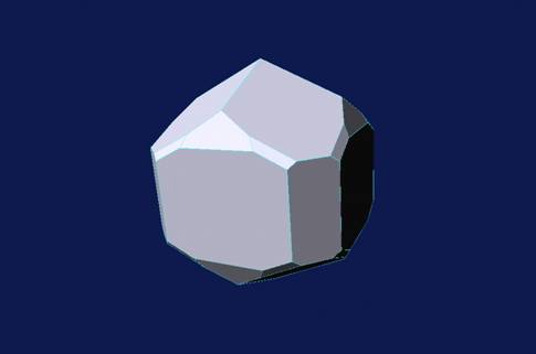
The code does make a number of assumptions, which should be removed before the production version is released. Perhaps the most important is that if the space group is A, B, C, I or F centred, then Space must be followed by FULL otherwise the index refers to the reduced unit cell. The second is that unlike the surface module in METADISE the particle generator does nothing to construct sensible surface terminations. Essentially, as with METADISE we will have to learn the rules.

One of the initial tests will be the use of the surface module to calculate all the relevant surface energies and hence construct a Wulff plot. The idealised total surface energy can now be compared with that calculated explicitly by generating a nanoparticle. The second part of the input gathers information about the nanoparticle by starting with the keyword nano and finishing with ends. The approach is then to use the Wulff plot to define a portion of space containing the nanoparticle and then fill the space with atoms defined by the crystallographic coordinate file using the rules defined within the nano/ends keywords.

The keywords are explained with examples
(ref: tio2_run1_1.met)
CUTO 1.000 25.85 0.5 60.0 60.0 1.0
LATT
4.492950999025 0.000000000000 0.000000000000
0.000000000000 4.492950999025 0.000000000000
0.000000000000 0.000000000000 3.008564956058
BASI
TI CORE 0.000000000000 0.000000000000 0.000000000000
TI CORE 2.246475499512 2.246475499512 1.504282478029 0
O CORE 1.362648117230 1.362648117230 0.000000000000
O 3.130302881795 3.130302881795 0.000000000000
O CORE 0.883827382283 3.609123616742 1.504282478029
O CORE 3.609123616742 0.883827382283 1.504282478029
ENDS

POTE

SPEC
O CORE -1.098 16.0
Ti CORE 2.196 47.88
ENDS
BUCK TI CORE O CORE
16957.53 0.194 12.59 100
ENDS
BUCK TI CORE TI CORE
31120.2 0.154 5.25 100
ENDS
BUCK O CORE O CORE
11782.76 0.234 30.22 100
ENDS

ENDS

surface
start
gem
space P42/mnm 136 1
index 1 0 0 2.082
index 1 1 0 1.77
index 0 0 1 2.406
index 0 2 1 2.283
index 1 2 1 2.11
index 0 1 1 1.85
index 2 2 1 2.02
nano
rad1 7.0
#scale 3.0
ends
start
stop

This will generate a simulation cell bounded by the symmetry related surfaces specified by index keywords. The input is converted to P1 symmetry and output as p1indices.res, which can then be used as a replacement for the input to the gem module and allows us make subtle changes to the morphology.

The coordinates of this run are all put into region 1 (as specified by rad1 which gives the limit of the most distant vertex). The alternative approach is to scale the morphology by a factor specified by scale, i.e. the conversion to Angs.

The output gives a table with ion type, coordinate, cumulative charge and the position number in the list. The position numbers can now be selected to give a neutral particle that can then be minimised. The following causes a 99 atom particle will be minimised.

ref: tio2_run1_2.met
....
gem
space P42/mnm 136 1
index 1 0 0 2.082
index 1 1 0 1.77
index 0 0 1 2.406
index 0 2 1 2.283
index 1 2 1 2.11
index 0 1 1 1.85
index 2 2 1 2.02
nano
rad1 7.0
nat1 99
#scale 14.0
ends
start
minimise
conj 50
bfgs 100
STOP

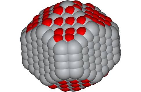
But this can easily to adjusted to minimise larger and larger particles. Note for small particles, any molecular viewer will do the job.

2.6 nm rutile nano-particle

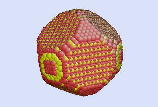
For larger particles, it looks like Atom-eye is a good display viewer. It is only available for Linux, but can display and manipulate many atoms. For example the following shows an image of a 20 nm particle with over 36000 species.

20 nm nano particle of ceria, showing both polar and non-polar surfaces

An alternative way of using the code is to use a 2 region approach, i.e. holding one set of ions fixed (region 2) and allowing the other ions to relax (region 1). In this example a simulation cell is generated with the inner, 9 atom, portion allowed to relax and the outer (region 2) held fixed.

ref tio2_run2_2.met
...
...
nano
rad1 7.0
nat1 9
nat2 99
#scale 14.0
ends
start
minimise
conj 50
bfgs 100
STOP

In the following example the ions in the outer region are free to relax and the ions in the inner portion are held fixed. This is achieved by first approximately setting up the region sizes,

ref:tio2_run4_1.met
....
....
nano
rad2 4.0
rad1 7.0
#scale 14.0
ends
start
STOP

note that the region 1 is bigger. Inspection of the output shows that it is not charge neutral:

ref:tio2_run4_2.met
....
space P42/mnm 136 1
index 1 0 0 2.082
index 1 1 0 1.77
index 0 0 1 2.406
index 0 2 1 2.283
index 1 2 1 2.11
index 0 1 1 1.85
index 2 2 1 2.02
nano
rad2 4.0
rad1 7.0
nat2 12
nat1 66
#scale 14.0
ends
start
minimise
conj 50
bfgs 50
start
STOP

nat2 12, causes the first 12 atoms to be associated with region 2, and atoms from 13 to 66 will be the new region 1. Again both are charge neutral.

Remaining considerations include automatically making the particle charge neutral. Although still incomplete, you could try adding the charge keyword.

Alternatively, the nanocrystal could be setup with reg1=4 and reg2=7, i.e. the fixed region will be in the inner region.

The test examples run so far seem to show that you have complete ion shells then the nanoparticle will most likely be non-polar but charged, If the outer shell is cut to maintain charge neutrality. The consequence is that the particle becomes polar. Thus there is still the question of how to select the positions of the incomplete outer shell of atoms.

Another potential use is to study the interaction between particles, by constructing particles and adding them together.

ref: tio2_run1_3.met

....
....
nano
rad1 7.0
nat1 99
chi 60.
phi 45.
theta 60.
shift 3. 6. 7.
ends
start
minimise
conj 50
bfgs 100
start
STOP

where shift, chi, phi and theta and the coordinate shift and rotations of the particle. Then the bef###.res files of the two particles can be combined to give a cell of the 2 particles.

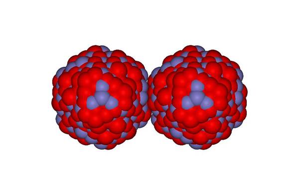
Here are two hematite particles generated using this approach. In addition, the keyword sphere is added after nano, forcing the code to generate spherical particles. Note, with the print dlpoly keyword, a DL_POLY dataset can be generated.

Two 2nm hematite particles

Summary list of keywords of GEM

After gem can have:

start
causes the module to start

cell # # # # # #
can enter a new set of cell dimensions (3 lengths followed by 3 angles)

space {full/redu} # # #
space group, give name, number and origin setting

latt
# # #
# # #
# # #
3 cartesian lattice vectors

index # # # #
3 Miller indices followed by surface energy

print # #
usual print statement

nano
causes the program to generate a nanoparticle

THE FOLLOWING COMMANDS CAN ONLY BE ENTERED AFTER nano

ends
to finish entering nanoparticle input – returns commands to GEM

cent # # #
x,y,z cartesian coordinate in unit cell, which will correspond to the centre of the particle
(Locating the centre seems to be an issue, to help to overcome this added a keyword; scan # # (will adjust centre by first amount for a number of times, e.g. scan 0.2 10 will scan in x,y and z directions between 0 and 2A in 0.2)
A nano_o###.res file will be generated with all the configurations.
setcharge # will save those configurations where the net charge is #)

shif # # #
shift whole particle by x,y,z

thet #
phi #
chi #
rotation angles about x, y and z axes, performed on whole particle – using the Goldstein convention.

expand # # #
Scales all coordinates in the different directions – allowing the crystal to be put under extension or tension

scale #
convert of surface energy to Angstroms

rad1 # (or reg1 #)
radius of region 1 (an alternative to scale)

rad2 # ( or reg2 #)
radius of region 2 (an alternative to scale)

nat1 #
explicitly set number of ions in region 1

nat2 #
explicitly set number of ions in region 2

sphere
ignores the index keywords when generating particle, thus gives a spherical particle.

fixcharge {nearly}
adjusts outer region so that particle is zero charged. {nearly} adjusts outer region to the last inflection in charge i.e. where it passes through zero.

dipole
not yet implemented – but idea is to remove dipole

Back to top

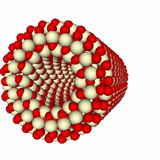
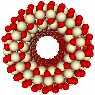
WRAP
The aim of this module is to create nanotubes. The procedure is start from a rotated unit cell. The simulation cell is then extended along the first vector – which lies along y. The third vector, which is the x-direction describes the exposed surfaces of the tube. Thus the exposed surfaces are the same as for the flat surfaces, specified by a Miller index and have a certain thickness, given by the region size. The cell is assumed to repeat in the z-direction, as given by the second lattice vector.
The simulation takes x=0 as the zero strain radius. This can be modified by using cent #, where # is a negative number to move the position of the zero strain radius.
A typical simulation cell:
print rough 0
cutoff 1.00000 15.00000 0.50000 60.00000
surf
region 3.00000 0.00000 3.00000 0.00000
stack
# This cell is PRE-ORIENTATED!
LATT (area = 12.764)
0.0000000000 3.8390746678 0.0000000000
0.0000000000 1.9195373339 3.3247361894
3.1345913402 1.9195373339 1.1082453965
Miller 1 1 1
code 1
BASI
O CORE 0.0000000000 5.7586120017 3.3247361894
O SHEL 0.0000000000 5.7586120017 3.3247361894
CE CORE 0.7836478351 1.9195373339 1.1082453965
O CORE 1.5672956701 3.8390746678 2.2164907929
O SHEL 1.5672956701 3.8390746678 2.2164907929
ends
Potential
SPEC
CE CORE 4.00000 140.11500
O CORE 0.830000 15.99940
O SHEL -2.8300 .00000
CA CORE 3.00000 140.11500
ends
BUCK
O SHEL O SHEL 22764.30000 .14900 27.89000
CE CORE O SHEL 1986.83000 .3511 20.40000
O SHEL CA CORE 1731.61808 .36372 14.43256
ENDS
HARM O CORE O SHEL 257.89000
ENDS
surf
vscale1
13.0 0.0
-1.0 2.0
charge
start
wrap
#reduce 2.0
radius 7.82
#length 49
#twist 3.2
strain
fill
rmin 1.61
#number 4
#
#bfgs 300
start

stop

Note: vscale1 is used to make a strip in the y-direction for the first vector and the second vector is converted into the form 0,0,z.
The resulting input file gives


Nano tube of ceria. The exposed surfaces are (111)

Summary of Keywords
Strain #
Compresses outer atoms so that make close contact (rather than default, which is even spacing). Does not need number (#). Default is 1.0, and if set to 0.0 it is as if the keyword was not entered.
Fill
If strain set, then fills outer layers with atoms to make complete rings
Number #
If strain and fill set, this increases the number of image cells.
Ring #
If strain and fill set, this sets how far round the ring the image cells go (1.0 means 2pi radians, if there is a gap at the join, then 1.05 will often fill it.

Length #
Allows user to specify circumference in Angs (default is for a complete ring). Enables U-shaped wires to be generated
Radius #
Similar to above but allows user to specify radius of tube in Ang
Rmin #
Minimum contact distance in Ang. Prevents atoms at join from overlapping
Twist #
Allows the tube to have a helicity. The distance in Angs, represents the shift along the z-direction of 2p rotations
Reduce #
Specifies the rate of reduction (or expansion) of the ring with length in the y-direction. Used to make spirals
Start
Begin the simulation

Note: can also include minimisation keywords, so as to minimise the simulation cell.

Back to top

Stop
As the name implies, this causes the program to stop and produces a XXXX####fin.res file which contains the coordinates and can be used for restarting.
Back to top

TITLE
Cr2O3 cell new pot
THIS RUN IS A RESTART OF THE
DATA SET WRITTEN AT ******** ON 04-Mar-9 RUN TIME = 37.69 S
TOTAL PREVIOUS RUN TIME: 37.69 S
ENDS
DIME 200000
JOBT 1000
PRIN PHON 0 MINI 0 BASI 2 BOND 2
THERM
CUTO 1.0 13.45 0.78 60.0 60.0 1.0
LATT
5.023953202229 0.000000000000 0.000000000000
-2.511976601114 4.350871100554 -0.000000000066
0.000000000000 0.000000000200 13.099124304710
BASI
CR CORE 0.000000000000 0.000000000069 4.551945695887 0
CR CORE 0.000000000000 0.000000000024 1.749595829777 0
CR CORE -0.000000000001 0.000000000124 8.299157982132 0
CR CORE -0.000000000001 0.000000000169 11.101507848242 0
CR CORE 2.511976601114 1.450290366987 8.918320464101 0
CR CORE 2.511976601114 1.450290366942 6.115970597992 0
CR CORE 2.511976601114 1.450290367042 12.665532750347 0
CR CORE 2.511976601114 1.450290366888 2.368758311746 0
CR CORE 0.000000000000 2.900580733706 0.185570927606 0
CR CORE 0.000000000000 2.900580733861 10.482345366206 0
CR CORE -0.000000000001 2.900580733761 3.932783213852 0
CR CORE -0.000000000001 2.900580733806 6.735133079961 0
O CORE 1.456475518485 0.000000000047 3.150770762832 0
O CORE -0.728237759242 1.261344799045 3.150770762813 0
O CORE 3.567477683743 0.000000000147 9.700332915187 0
O CORE 1.783738841872 3.089526301603 3.150770762784 0
O CORE -1.783738841873 3.089526301703 9.700332915139 0
O CORE 0.728237759242 1.261344799145 9.700332915168 0
O CORE 3.968452119600 1.450290366965 7.517145531047 0
O CORE 1.783738841872 2.711635165963 7.517145531028 0
O CORE 1.055501082628 1.450290366865 0.967583378692 0
O CORE 1.783738841872 0.188945567967 7.517145531065 0
O CORE 3.240214360356 0.188945567867 0.967583378710 0
O CORE 3.240214360356 2.711635165863 0.967583378673 0
O CORE 1.456475518485 2.900580733883 11.883520299261 0
O CORE -0.728237759242 4.161925532881 11.883520299242 0
O CORE -1.456475518486 2.900580733783 5.333958146906 0
O CORE -0.728237759242 1.639235934885 11.883520299280 0
O CORE 0.728237759242 1.639235934785 5.333958146925 0
O CORE 0.728237759242 4.161925532781 5.333958146887 0
CR SHEL 0.000000000000 0.000000000070 4.573682652552 0
CR SHEL 0.000000000000 0.000000000024 1.727858873112 0
CR SHEL -0.000000000001 0.000000000124 8.277421025467 0
CR SHEL -0.000000000001 0.000000000170 11.123244804907 0
CR SHEL 2.511976601115 1.450290366988 8.940057420767 0
CR SHEL 2.511976601115 1.450290366942 6.094233641326 0
CR SHEL 2.511976601113 1.450290367042 12.643795793681 0
CR SHEL 2.511976601113 1.450290366888 2.390495268412 0
CR SHEL 0.000000000000 2.900580733706 0.207307884272 0
CR SHEL 0.000000000000 2.900580733860 10.460608409541 0
CR SHEL -0.000000000001 2.900580733760 3.911046257186 0
CR SHEL -0.000000000001 2.900580733806 6.756870036626 0
O SHEL 1.457957860760 0.000000000047 3.150770762832 0
O SHEL -0.728978930380 1.262628545112 3.150770762813 0
O SHEL 3.565995341468 0.000000000147 9.700332915187 0
O SHEL 1.782997670734 3.088242555536 3.150770762784 0
O SHEL -1.782997670735 3.088242555636 9.700332915139 0
O SHEL 0.728978930379 1.262628545212 9.700332915168 0
O SHEL 3.969934461875 1.450290366965 7.517145531047 0
O SHEL 1.782997670734 2.712918912030 7.517145531028 0
O SHEL 1.054018740353 1.450290366865 0.967583378692 0
O SHEL 1.782997670734 0.187661821900 7.517145531065 0
O SHEL 3.240955531494 0.187661821800 0.967583378710 0
O SHEL 3.240955531494 2.712918911930 0.967583378673 0
O SHEL 1.457957860760 2.900580733883 11.883520299261 0
O SHEL -0.728978930380 4.163209278948 11.883520299242 0
O SHEL -1.457957860761 2.900580733783 5.333958146906 0
O SHEL -0.728978930380 1.637952188818 11.883520299280 0
O SHEL 0.728978930379 1.637952188718 5.333958146925 0
O SHEL 0.728978930379 4.163209278848 5.333958146888 0
ENDS
POTE
SPEC
O SHEL -2.18 0.0
O CORE .18 15.9994
CR CORE 2.03 52.996
CR SHEL 0.97 0.0
ENDS
BUCK O SHEL CR SHEL
1734.1 0.3010 0.0
ENDS
BUCK O SHEL O SHEL
22764.3 0.1490 27.99
ENDS
HARM O CORE O SHEL 27.29
HARM CR CORE CR SHEL 100.00
ENDS
region 1.0 1.0 10.0 10.0
conp
START
STOP

# experimental data
# minimise bulk crystal structure
title
calcite
ends
dime 180000
prin reg1 1
maxi 20
cuto 1.0 10.10 0.8 60.0 60.0
cell 4.9896 4.9896 17.0610 90.0 90.0 120.0
space reduce r3-ch 167 1
frac
ca core 0.0000 0.0000 0.0000
c core 0.0000 0.0000 0.2500
o core 0.2568 0.0000 0.2500
o shel 0.2568 0.0000 0.2500
ends
pote
spec
ca core 2.0 40.0
c core 1.135 12.0
o core 0.587 16.0
o shel -1.632 0.0
ends
buck o shel o shel
16372.0 0.213 3.47 20.0
ends
buck ca core o shel
1550.0 0.297 0.0 20.0
ends
mors c core o shel
4.71 3.80 1.18 0.0 1.4
ends
harm o core o shel 507.4
boha 1 1.69 120.0
toha 1 0.11290 1 2
ends
thbo
anga 1 c core o core o core
1.4 1.4 2.4
ends
tors
tora 1 c core o core o core o core
rij max 1.4
rik max 1.4
ril max 1.4
rjk max 2.4
rjl max 2.4
rkl max 2.4
ends
maxi 100
maxu 10
conp
stop
start
stop

# fin####.res file contains relaxed coordinates
#modify so that it can locate 104 surface
title
calcite
ends
dime 180000
prin reg1 1
maxi 20
cuto 1.0 10.10 0.8 60.0 60.0
CELL 4.796789 4.796789 17.481955 90.0000 90.0000 120.0000
space reduce r3-ch 167 1
FRAC
CA CORE .0000000000000 .0000000000000 .0000000000000
C CORE .0000000000000 .0000000000000 .2500000000000
O CORE .2492017811563 .0000000000000 .2500000000000
O SHEL .2481191122287 .0000000000000 .2500000000000
ends
pote
spec
ca core 2.0 40.0
c core 1.135 12.0
o core 0.587 16.0
o shel -1.632 0.0
ends
buck o shel o shel
16372.0 0.213 3.47 20.0
ends
buck ca core o shel
1550.0 0.297 0.0 20.0
ends
mors c core o shel
4.71 3.80 1.18 0.0 1.4
ends
harm o core o shel 507.4
boha 1 1.69 120.0
toha 1 0.11290 1 2
ends
thbo
anga 1 c core o core o core
1.4 1.4 2.4
ends
tors
tora 1 c core o core o core o core
rij max 1.4
rik max 1.4
ril max 1.4
rjk max 2.4
rjl max 2.4
rkl max 2.4
ends
surface
# add region and miller index
region 1 1 1 1
miller 1 0 4
maxi 100
maxu 10
# delete next 2
#conp
#stop
start
#add stackgen bits
stackgen systematic
coor c core o core 1.4
coor c core o shel 1.4
start
stop

title
calcite
ends
dime 180000
prin reg1 1
maxi 20
cuto 1.0 10.10 0.8 60.0 60.0
CELL 4.796789 4.796789 17.481955 90.0000 90.0000 120.0000
space reduce r3-ch 167 1
FRAC
CA CORE .0000000000000 .0000000000000 .0000000000000
C CORE .0000000000000 .0000000000000 .2500000000000
O CORE .2492017811563 .0000000000000 .2500000000000
O SHEL .2481191122287 .0000000000000 .2500000000000
ends
pote
spec
ca core 2.0 40.0
c core 1.135 12.0
o core 0.587 16.0
o shel -1.632 0.0
ends
buck o shel o shel
16372.0 0.213 3.47 20.0
ends
buck ca core o shel
1550.0 0.297 0.0 20.0
ends
mors c core o shel
4.71 3.80 1.18 0.0 1.4
ends
harm o core o shel 507.4
boha 1 1.69 120.0
toha 1 0.11290 1 2
ends
thbo
anga 1 c core o core o core
1.4 1.4 2.4
ends
tors
tora 1 c core o core o core o core
rij max 1.4
rik max 1.4
ril max 1.4
rjk max 2.4
rjl max 2.4
rkl max 2.4
ends
surface
region 1 1 1 1
miller 1 0 4
maxi 100
maxu 10
start
# replace systematic by an index cut - see also pldraw####
#stackgen systematic
stackgen 1
coor c core o core 1.4
coor c core o shel 1.4
start
stop

# minimise rotated unit cell
title
calcite
ends
dime 180000
prin reg1 1
maxi 20
cuto 1.0 10.10 0.8 60.0 60.0
stack
# This cell is PRE-ORIENTATED!
LATT
#CELL 4.796789 4.796789 17.481955 90.0000 90.0000 120.0000
.0000000000 4.7967890000 .0000000000
.0000000000 .0000000000 8.0396860576
3.0110010013 -2.3983945000 -2.8619506465
# space reduce r3-ch 167 1
BASI
C CORE .1000000000000 4.7967890000000 7.1876569255203
O CORE -.6503468125837 4.1991048186845 7.9008601242160
O SHEL -.6470868953586 4.2017014858858 7.8977615791787
O CORE .1000000000000 5.9921573626310 7.1876569255203
O SHEL .1000000000000 5.9869640282284 7.1876569255203
O SHEL .8470868953586 4.2017014858858 6.4775522718619
O CORE .8503468125836 4.1991048186845 6.4744537268246
CA CORE .1000000000000 2.3983945000000 5.1777354111110
CA CORE .1000000000000 2.3983945000000 1.1578923822925
C CORE .1000000000000 4.7967890000000 3.1678138967018
O CORE -.6503468125836 5.3944731813155 3.8810170953975
O SHEL -.6470868953586 5.3918765141142 3.8779185503602
O CORE .1000000000000 3.6014206373691 3.1678138967018
O SHEL .1000000000000 3.6066139717716 3.1678138967018
O SHEL .8470868953586 5.3918765141142 2.4577092430434
O CORE .8503468125837 5.3944731813155 2.4546106980060
#fractional
#CA CORE .0000000000000 .0000000000000 .0000000000000
#C CORE .0000000000000 .0000000000000 .2500000000000
#O CORE .2492017811563 .0000000000000 .2500000000000
#O SHEL .2481191122287 .0000000000000 .2500000000000
ends
pote
spec
ca core 2.0 40.0
c core 1.135 12.0
o core 0.587 16.0
o shel -1.632 0.0
ends
buck o shel o shel
16372.0 0.213 3.47 20.0
ends
buck ca core o shel
1550.0 0.297 0.0 20.0
ends
mors c core o shel
4.71 3.80 1.18 0.0 1.4
ends
harm o core o shel 507.4
boha 1 1.69 120.0
toha 1 0.11290 1 2
ends
thbo
anga 1 c core o core o core
1.4 1.4 2.4
ends
tors
tora 1 c core o core o core o core
rij max 1.4
rik max 1.4
ril max 1.4
rjk max 2.4
rjl max 2.4
rkl max 2.4
ends
surface
#increase region - must check convergence
region 4 4 40 40
miller 1 0 4
maxi 100
maxu 10
start
#remove stackgen - replace with minimise
#stackgen 1
#coor c core o core 1.4
#coor c core o shel 1.4
#start
minimise
conj 20
newt 30
start
stop

Back to top

Contact Information
Electronic mail: s.c.parker@bath.ac.uk
Address: Dept. of Chemistry, University of Bath, Bath, BA2 7AY, U.K.
Web address: http://www.bath.ac.uk/~chsscp/group
Telephone: - 44 (0) 1225 386505
Last Revised: 22 Sept 2003

METADISE 5.15

Minimum Energy Technique Applied to Dislocation, Interface and Surface Energies

Modules in the Metadise Code

Meta, Property, Stackgen, Miller, Step, Minimise, Flexible, Scan, IR, MD, MC, Phon Match Chaos Segregate GEM Wrap and Stop

Stop

Are under development. Segregate

Further Information on the Metadise Code

Metadise Input Controller

Keywords:

Control Keywords which modify the Simulation Cell Generated

Control Keywords used to manipulate block2 coordinates with respect to block1

Control keywords for adding further species to simulation cell

Control Keywords relating to printing

Control Keywords relating to Simulation of Crystal Structure

Crystal Structure:

Unit Cell input:

Lattice vectors

Basis Coordinates

Crystallographic:

Unit Cell Dimensions

Space Group

Fractional Coordinates

Restart input:

Surface Lattice vectors or Burgess vector

Surface Basis Coordinates

Either

Potential Model Controller Keywords

1. species

2. two body potentials

3. many body

4.

ends

5. Additional cutoff data for many-body terms

Keywords for original Metastar program: time, rest, debug, dump, in22

General:

for Newton Raphson

for Conjugate Gradients

for BFGS

Are under development.

Segregate