Parabolic Equation Modelling Dr Robert Watson, Department of Electronic & Electrical Engineering, University of Bath

Parabolic Equation Modelling for tropospheric propagation prediction

Parabolic equation model (PEM) techniques have been extensively used for radio propagation studies for more than twenty years. One of their main uses is an aid to the userstanding of the propagation of VHF, UHF and microwave signals. In particular PEM allows the study of the interation of EM waves with complex terrain and refractive index conditions. My interest in PEM techniques is with regard to work in passive radar and signals of opportunity for remote sensing.

Some examples of PEM output

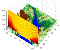
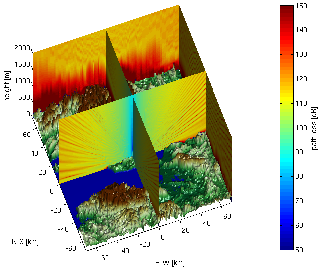
The model outputs here are from the PEM model described by M. Levy, "Parabolic equation methods for electromagnetic wave propagation", using terrain data taken from the SRTM (Space Shuttle Radar Topography Mission). The outputs show the propagation path loss for signals from an omnidirectional antenna located at the origin (0,0), approximately the location of the 222.064 MHz DAB transmissions from Wenvoe in Wales. Two orthogonal slices are shown at (0,0) along the East-West and North-South directions. The loss is also shown on two of the boundary walls. You can clearly see the huge diffraction (shadowing) losses caused by the Brecon Beacons - similar losses are seen if you "look" the other way over Exmoor

Here are some animations of various slices through the PEM derived output (warning some of these files are quite large)

1. East-West slices through domain - you can see clearly see losses due to Brecon Beacons and Exmoor (~2Mb).
2. North-South slices through domain - you can see the low loss over the Severn Estuary (~2Mb).
3. Vertical slices over the whole domain: large (~10Mb) and small (~6Mb) - can clearly see the diffraction shadowing caused by the terrain.
4. Rotated view over the whole domain: large (~25Mb) and small (~20Mb).