 Swiss-Model, one of many bioinformatics tools
available on http://www.expasy.org/.
Swiss-Model, one of many bioinformatics tools
available on http://www.expasy.org/.Once a novel protein has been sequenced, its function and the important functional residues needs to be determined. Bioinformatics cannot provide a definitive function for a protein, as any hypothesis needs to be confirmed in the laboratory, but it can provide indications of possible functions through primary, secondary or tertiary structure similarity with proteins of known function.
Predicting the tertiary structure of proteins from primary sequence alone is a Holy Grail of bioinformatics, but although this has been the subject of intense research effort for many years, it is not yet possible. However new structures often have a similar fold to others already in the database, so methods have been devised to model structure on the basis of known folds. The simplest is ‘Homology Modelling’ where the sequence of the unknown is aligned to that of a known structure and then that known structure is used to predict the fold of the unknown. As a general rule, the identity between the query and template sequences needs to be greater than 25% across the complete alignment for a useful model. If there is less similarity, a fold may still be identified by a process called ‘Threading’ where the sequence is ‘threaded’ into the shape of each of a library of known folds which are then scored based on compatibility (e.g. does the resulting model have features of a normal folded protein such as a hydrophobic core).
In this workshop we’ll work with the sequence of a protein involved in signalling in Arabidopsis thaliana to illustrate the modelling process. This is a short sequence, and the structure doesn't have much secondary structure, which is often used to judge the quality of a model but being short means that the modelling will run within the workshop time. This protein is known to have four disulphide bonds, and we will use this as another marker for model quality.
1. Submission of sequence to Swiss-model for Homology Modelling
2. Using a structure with similar function as template
3. Optimising the sequence alignment for homology modelling
4. Using an optimised alignment in homology modelling
5. Model validation and structure comparison
Homology or more strictly ‘Comparative’ modelling, builds the 3D structure of a protein of known sequence but unknown structure based on that of a protein with similar sequence and known structure. This process is critically dependent on the quality of the alignment between the two sequences and for this reason can only be carried out between two proteins of relatively high sequence identity (>25%).
The sequence of the A.thaliana protein is:
>At_alpha
SSLYFAILCLFMIFLVPLHEFGNAQGSEAELQLDPSMCLRVECAKHRNQKWCFCCAGLPRTCFLDKRGCTSVCKRESPSMA
One of the more straightforward comparative modelling servers
is
Swiss-Model, one of many bioinformatics tools
available on http://www.expasy.org/.
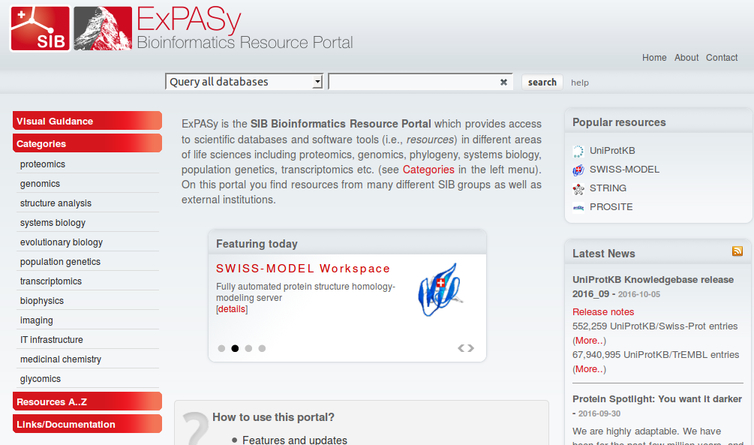
You can find Swiss-Model either under Resources A..Z on the left-hand side, or from the Popular resources menu on the right-hand side. A detailed protocol for using this site has been published in Nature Methods.
On the Swiss-Model page, click on the Start Modelling button.
This brings up a Start a New Modelling Project window. Copy the sequence from this script into the Target Sequence box.
Give your model a title, such as Model 1 and put in your email address. Then click Build Model
A new page appears, which is updated until your modelling is complete.
At the top of the new page are 3 hyperlinks, Summary,Templates and Models.
Start by clicking on Summary
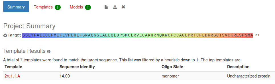
In this Project Summary we can see that 7 structures matched our sequence, which were automatically filtered down to 1. The sequence identity is very low, only 14% which means that our model is unlikely to be very good without manual intervention.
Moving on to the Templates page, there is a graphical view of the coverage of our sequence by the selected protein.
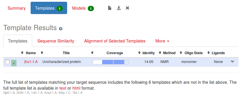
The blue bar indicates the part of our sequence that will be modelled.This is only part of the protein's total length, another indication that this round of modelling might not be very good, although in fact the first part is a signal peptide, so not part of the expressed protein, so we would not expect it to be modelled. However the sequence identity between the two sequences is only 14%, which is poor.
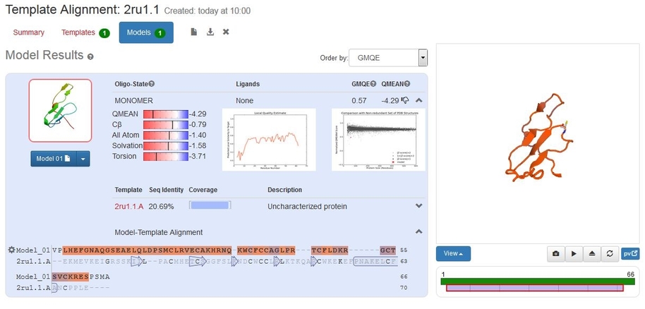
Finally the Models window. This shows our model, with some indications as to its reliability. The GMQE, the Global Model Quality Estimation, assesses the reliability of the whole model (a more detailed explanation can be found by clicking on the ? following each term) ranging from 0 to 1 where higher is better, so 0.32 is poor. QMEAN is a scoring function for estimating the model quality, where larger numbers are an indication of a better model.
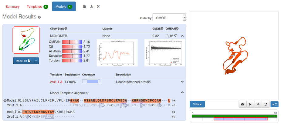
The model (shown above) covers about 2/3 of the sequence (as shown in the graphic below the cartoon of the model). In the blue box are various estimations of the quality of the model, compared to structures in the PDB database.
In the red-blue scales you can see that this model, shown by the black line, is less good (more red) than the average. This is also shown in the graph of QMEAN4 against protein size, where our model shows up as a red star. However very small structures like this do have a wide variation in QMEAN4 anyway.
To look at the structure, you could use the pv viewer on the right-hand side. This viewer allows you to rotate the image and to zoom in by scrolling the wheel.
To use a more powerful viewer, download the model by clicking on the Model 01 button on the left-hand side, (or on the download arrow next to it and choosing PDB File ). This downloads the model to your browser. Save it to your computer and double click on the file.
The default PDB viewer on BUCS computers is PyMOL, a very powerful picture-drawing package, and also quite complicated. If it doesn't open automatically, search for it from the Windows Start menu. If this happens you will need to Open (from the File menu) the file. When the structure is visible in the larger window, you can rotate it with the left-hand mouse button. Pull-down menus to change the picture are accessed under the letters at the top right of the view.
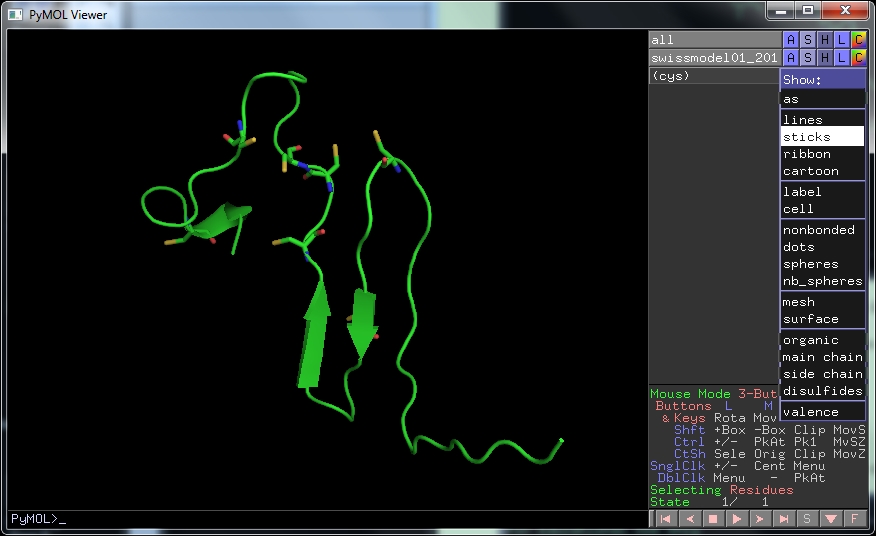
 First click on H , the Hide menu, then lines to remove the lines. Then click on
S , the Show menu, and
cartoon , to show the molecule with secondary structure.
First click on H , the Hide menu, then lines to remove the lines. Then click on
S , the Show menu, and
cartoon , to show the molecule with secondary structure.
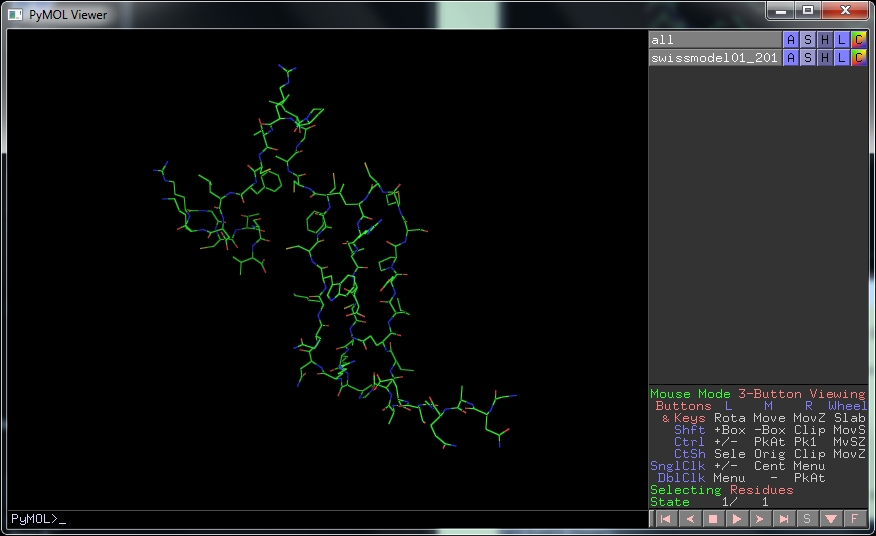
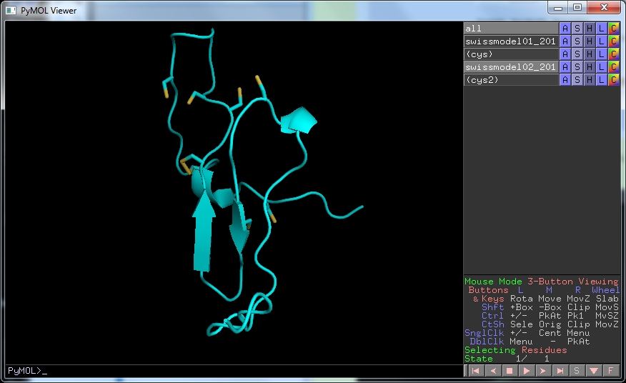
Now it should look as on the Swissmodel page. The 8 Cys residues in this protein are supposed to form four disulphide bonds. To show the cysteine residues in the protein, type
select cys, resn cys
after the PyMOL prompt in the window above.
A new line appears on the lower window. In this new line click on S , then sticks to show the cysteine residues.
By rotating the structure you can see that none are involved in disulphide bonds. Clearly this model isn't good enough to predict the structure.
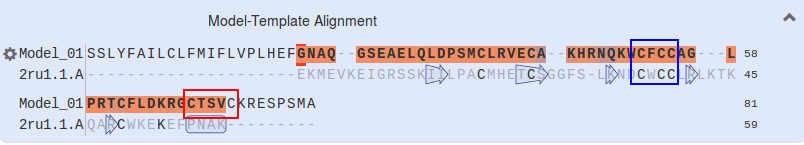
Looking at the alignment of our sequence with 2RU1, it is clear that several of the Cys (C) amino acids have been matched, in particular the CXCC motif in the middle. However towards the C-terminus there is a CXXXC motif which hasn't been aligned. We will try aligning this motif to see if this improves the model
To obtain the sequence of the 2RU1 protein, click on the 2ru1.1.A hyperlink just above the alignment. A new link opens with details of 2ru1, showing that it is involved in plant development and thus has a similar function to our peptide. Click on the cog at the left-hand side of the alignment, and then choose FASTA format at the top.
This brings up a new window showing the sequence, which we can copy directly into the sequence alignment window.
We will use T-coffee to align the sequences as we did in the previous workshop. Click on www.ebi.ac.uk, then on Services and on Proteins on the Services page, to find the T-Coffee link.
Put the sequence of our protein into the box, without the probable signal peptide i.e.
>At_alpha no signal peptideVPLHEFGNAQGSEAELQLDPSMCLRVECAKHRNQKWCFCCAGLPRTCFLDKRGCTSVCKRESPSMA
then the 2RU1 sequence that you have just downloaded. Then click the Submit button.
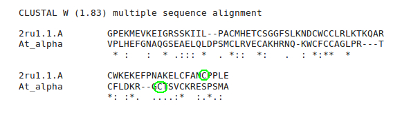
On the results page we can see that the alignment is very similar to that produced by Swiss-Model, i.e. the later Cys are still not aligned.
To edit the alignment, Download Alignment File and save it to a file. Read this file into SeaView as we did in workshop 2. Find the folder into which you downloaded SeaView and double click on the icon.
Click on File then Open to read in the alignment you saved.

Towards the C-terminus of the alignment, click on the - before the misaligned C in the sequence whose structure we are trying to model. Add more - to move the misligned C to the right until it lies above (or below depending on the order in which you aligned them in t-coffee) a C in the 2RU1 sequence. This also aligns the C-terminal pair of Cys.

Save the edited alignment as a new file
Now return to your Swiss-Model window, and go back to the beginning to Start a new Modelling Project.
This time select the Target-Template Alignment tab on the right-hand side of the page. Paste your alignment into the box.
Next you need to tell Swiss-Model which is the target (the sequence we're trying to model) and which the template (the sequence of the protein with known structure). Select the appropriate option (the template probably begins 2RU1_A), then click the Validate Target-Template Alignment button.
Once the alignment has been verified, click the Build Model .
On the Models window we can see that using our new alignment the sequence identity has increased to 20.7%, still on the low side, but better than before and the GMQE has increased to 0.57, although the QMEAN4 is worse.
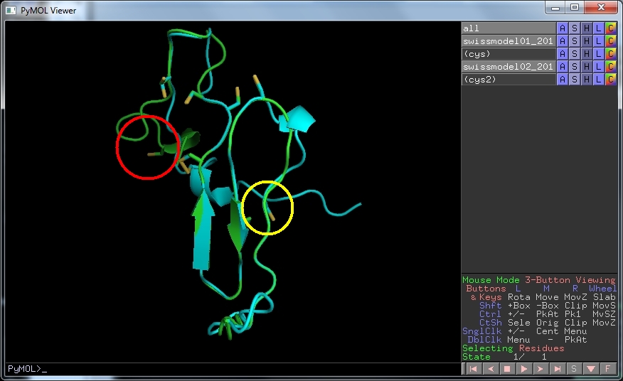
Download this structure and open it in PyMOL. As before, draw the cartoon representation and hide the lines. Select S , then disulfides and finally sticks to show the disulphide bonds.
We can see that the model now has one disulphide bond and that the other pairs of cysteine residues are in appropriate positions to make the remaining 3. Since the modelling used the edited sequence alignment, you can see that where one of the cysteines used to face into solvent (red circle) all are now in appropriate places (yellow circle). This is probably as reliable a structure as we can get with this small protein.
 For larger proteins, with more defined secondary structure elements, models with more than 25% sequence identity usually achieve much better QMEAN4 and GMQE values.
Having obtained a model of our protein by homology modelling, we need to analyse this model to see if we can determine whether it is reliable. Often such a model is used as the basis for subsequent experiments so we need to obtain a model which best fits our knowledge of the protein.
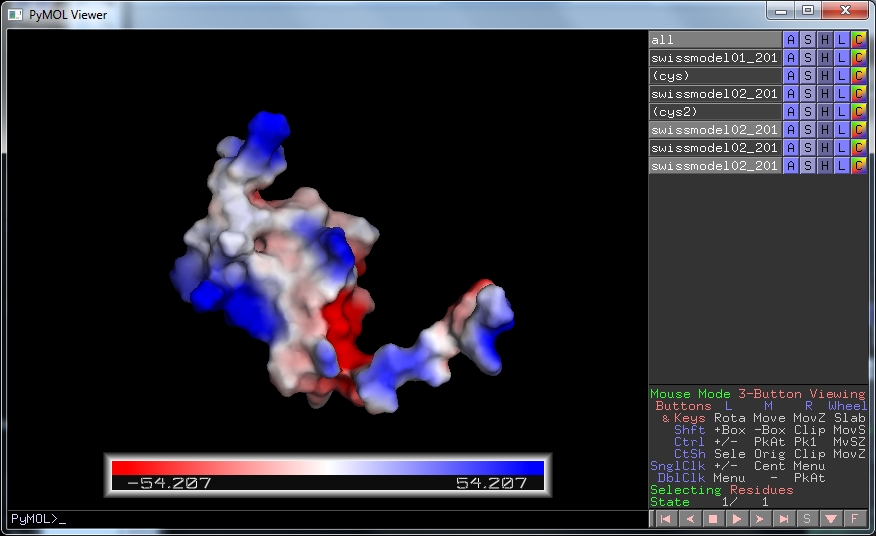
Firstly we would use any biological information we have about the protein to test whether the model agrees with this, as we have with the disulphide bonds throughout this workshop. Another feature about which we might know is the substrate or binding partner of the protein of interest. In particular we might know whether it is charged. To display the charged surface of our model in Pymol, click on A , then vacuum electrostatics and finally protein contact potential .
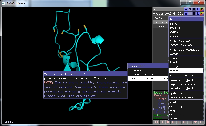 This shows the surface of the model coloured by electrostatic potential, red is negative, blue is positive. Some areas are exclusively negative, others positive, with one side more hydrophobic (less coloured) than the rest. This would be informative if you worked with these proteins.
Some automated validation was carried out by Swiss-MODEL itself. We will do one of the simplest validation procedures, calculating a Ramachandran plot. Ramachandran plotted the phi and psi angles of amino acids and noted that some areas of this phi-psi space were more favourable than others and some were disallowed due to clashes. There are many tools to calculate Ramachandran plots on the web. One of these is RAMPAGE: http://mordred.bioc.cam.ac.uk/~rapper/rampage.php
Here click Browse and find your final saved PDB file. Then SUBMIT TO RAMPAGE .
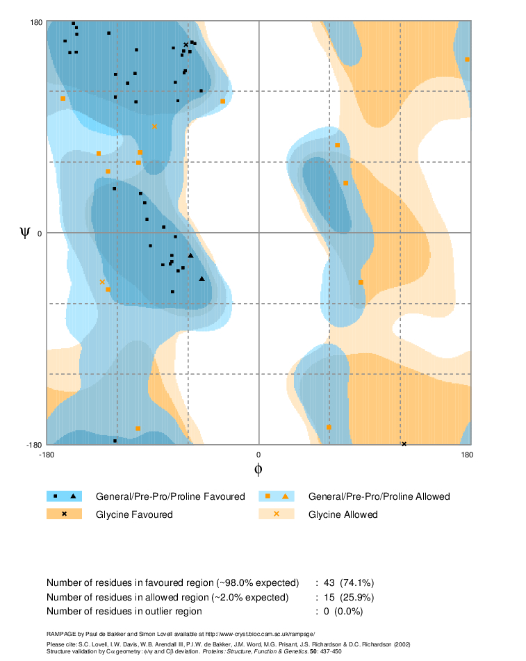
In the resulting plot, the most favourable amino acids are in the dark blue regions, allowed regions are in lighter blue, generously allowed in pale blue and disallowed in white. Glycine has more allowed regions due to its lack of a side chain, and is permitted in the dark and light orange regions as well. All residues in disallowed regions would be labelled, these are likely to be modelled incorrectly and indicate areas which need more work.
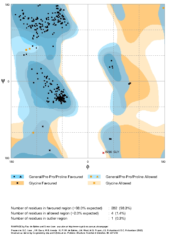
Overall statistics for our model are gathered at the bottom, you may need to scroll down the page. As it states, a good structure would be expected to have over 98% in favoured regions of the plot and this model has only 74.1%. This is worse that the structure from which it was modelled, 1RU1, although this does have one residue in a disallowed region.
If there was more time, to reduce the number of amino acids in the disallowed areas and increase those in the most favoured regions you would go back and alter the sequence/structure alignments on which they are based.
Apart from comparison with a known structure, having which would make a model redundant anyway, the only way of validating the model is by comparing it with the known biological function as we have been doing through the workshop.
If more structures were known, an overall alignment and comparison of two structures could be carried out using PDBeFold from the EBI Toolbox:
http://www.ebi.ac.uk/msd-srv/ssm, however in the case of the sequence we've used this isn't possible as there is only one. I have included this for completeness for those who generate homology models in their research.
This workshop has
produced a model through automated homology modelling methods.
It is always better to include biological knowledge
in the modelling process through careful production of a multiple
sequence alignment based on known structures and to use this to produce
a model. The best software available to do this at the moment is
 MODELLER,
which can be downloaded to your own computer and tailored to
your particular project.
MODELLER,
which can be downloaded to your own computer and tailored to
your particular project.
If there isn't a structure in the PDB that shares more than 20% sequence
similarity with the sequence you need to model, then Swiss-Model (and
other homology modelling programs) will not work. However it seems that there are only a
limited number of ways that a protein can fold into a 3D structure
and there is an ~70% chance that a newly-discovered protein will have
a similar fold to that of one already in the database. The
“threading” or “fold
recognition” method scores how well each
of the folds in the database would fit the target sequence to predict
a final model for a less similar protein. One of the best web-based programs available to do this is
 PHYRE
(Protein Homology/analogY
Recognition Engine)
server. Phyre takes considerably longer to run than Swiss-Model, so is less suitable for a workshop, (it took 20 minutes when I tried it), but
again the minimal input is just a sequence, so it is straightforward, and
the results can be compared with those from Swiss-Model using DaliLite
as above. For a protein as short as the one used in this workshop the results of the default Phyre modelling were not convincing, only modelling short stretches of the sequence, however for larger proteins it produces competitive models. More detailed instructions on how to run an optimal phyre run
are given here.
PHYRE
(Protein Homology/analogY
Recognition Engine)
server. Phyre takes considerably longer to run than Swiss-Model, so is less suitable for a workshop, (it took 20 minutes when I tried it), but
again the minimal input is just a sequence, so it is straightforward, and
the results can be compared with those from Swiss-Model using DaliLite
as above. For a protein as short as the one used in this workshop the results of the default Phyre modelling were not convincing, only modelling short stretches of the sequence, however for larger proteins it produces competitive models. More detailed instructions on how to run an optimal phyre run
are given here.